The breakthroughs in deep learning over the last decade have revolutionized computer image recognition.   The state-of-the-art deep neural networks have 10s of millions of parameters and they require training sets of similar size.   The training can take days on a large GPU cluster.   The most advanced deep learning models can recognize over 1000 different objects in images with surprising accuracy.   But suppose you have a computer vision task that requires that you classify a few dozen different objects.   For example, suppose you need to identify ten different subspecies of wolf, or different styles of ancient Korean pottery or paintings by Van Gogh?    These tasks are far too specific for any of the top-of-the-line pretrained models.  You could try to train an entire deep network from scratch but you if you only have a small number of images of each of your specialized classes this approach will not work.

Fortunately, there is a very clever technique that allows you to “retrain” one of the existing large vision models for your specific task.  It is called Transfer Learning and it has been around in various form from the mid 1990s.   Sebastien Ruder has an excellent blog that describes many aspect of transfer learning and it is well worth a read.

In this article we look at the progress that has been made turning transfer learning into easy-to-use cloud services.    Specifically, we will look at four different cloud services for building custom recognition systems.   Two of them are systems that have well developed on-line portal interfaces and require virtually no machine learning expertise.   They are the IBM Watson Visual Recognition Tool and Microsoft Azure Cognitive Services Custom Vision service.   The other two are tools that require a bit of programming skill and knowledge about deep networks.  These are the Google “Tensorflow for Poets” Transfer learning package and the Amazon Sagemaker toolkit.    To illustrate these four tools, we will apply each systems to the task of classifying images of galaxies.   The result is not deep from an astronomy perspective (because I am not even an amateur astronomer!), but it illustrates the power of the tools.   We will classify the galaxies into four types: barred spiral, elliptical, irregular and spiral as illustrated in Figure 1.     We will do the training with very small training sets:  19 images of each class that were gathered from Bing searches.

The classification task is not as completely trivial as one might assume.   Barred spiral galaxies are a subspecies of spiral galaxy that are distinguished by a “bar” of stars at the origin of the spirals.  Consequently, these two classes are easy to misidentify. Irregular galaxies can be very irregular.  (I like to think of them as galaxies that have not “got it together” enough to take on one of the other forms.)   And elliptical can often look like spiral or irregular galaxies.

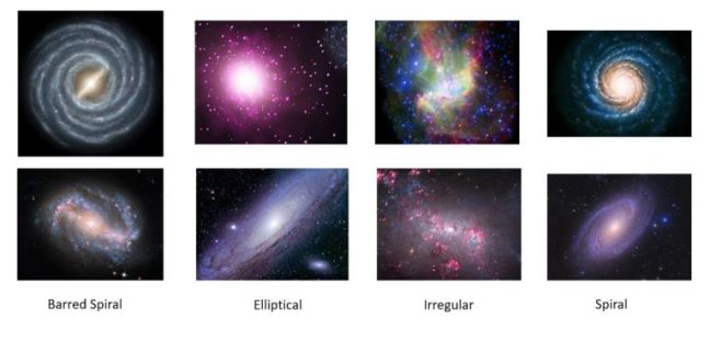
Figure 1.   Two samples each of the four galaxy types.  The images were taken from Bing searches.

We have made these image files available at AWS S3 in two forms: a zip files barred, elliptical, irregular, spiral and test and in REC format as galaxies-train.rec and galaxies-test.rec.

Transfer Learning for DNNs

Before we launch into the examples, it is worth taking a dive into how transfer learning work with a pre-built deep learning vision model.   A good example, and one we will use, is the Inception-V3 model shown in Figure 2.

Figure 2.  Inception-V3 deep network schematic.   Image from the Google Research blog “Train your own image classifier with Inception in TensorFlow“.

In  Figure 2, each colored blob is a subnetwork with many parameters.  The remarkable thing about deep networks is how much of lower layers of convolution, pooling, concatenation seem to capture abstract qualities of images such as shapes and lines and regions.  Suppose the network has L layers  At the risk of greatly oversimplifying one can say that it is only at the last few layers that specific image classification takes place.   A simple way to do transfer learning is to replace the last two layers with two new ones and retrain the trained parameters of layers 0 to L-2 “constant” (or nearly so).

The paper https://arxiv.org/pdf/1512.00567.pdf  “Rethinking the Inception Architecture for Computer Vision” by  Szegedy et al. describes InceptionV3 in some detail.   The last two layers are a fully connected layer with 2024 inputs and 1000 softmax outputs.     To retrain it for 4 outputs  we replace last layers as illustrated in Figure 3 with two new layers. We now have only one matrix W of dimension 2024 by 4 of parameters we need to learn

Figure 3.   Modified network for transfer learning.

If the training algorithm converges, it will be literally thousands of time faster than training the original.  A nice paper by Yosinski et al takes an in-depth look at feature transferability in deep networks.   There are other ways to do transfer learning on deep nets than just holding the L-2 layers fixed.   Instead one can allow some fine tuning of the top most layers with the new data.    There is much more that can be said on this subject, but our goal here is to evaluate some of the tools available.

The IBM Watson Visual Recognition tool.

This transfer learning service is incredibly easy to use.   There is an excellent drop-and-drag interface and a nodeJS API as well as a Python API.   To test it we clicked on the create classifier button and dragged the zip files for our four classes of galaxies onto the interface as shown below.

Figure 4. Visual recognition tool Interface with dragged zip files for the galaxy classes.

Within a few minutes we had a view of the classifier that we could test.   The figure below illustrates the results from dragging three examples from the training set to the classifier interface.  As you can see the interface returns the relative strength of membership in each of the classes.

To invoke the service, you need three things:

1. your IBM bluemix api_key which you were given when you logged into the service the first time to build the model.
2. Once your model has been built you need the classifier ID which is visible on the tool interface.
3. you must install the watson_developer_cloud module with pip.

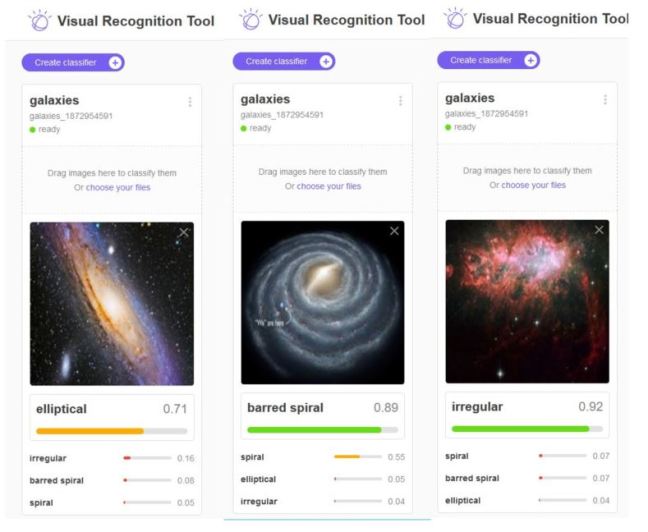
Figure 5:  Three vertical panels show the result of dragging one of the training images onto the classifier interface.

import watson_developer_cloud
from watson_developer_cloud import VisualRecognitionV3
visual_recognition = VisualRecognitionV3( 
      api_key = '1fc969d38 your key here 7f7d3d27334', 
      version = '2016-05-20')
classifier_id = 'galaxies_1872954591'
image_url = https://s3-us-west-2.amazonaws.com/learn-galaxies/bigtest/t12.jpg
   
param = {"url": image_url, "classifier_ids":[classifier_id]}
visual_recognition.classify(parameters=json.dumps(param)

The key elements of the code are shown above.  (There may be other versions of the Python API.  This one was discovered by digging through the source code.   There is little other documentation.)  We built a Jupyter notebook that uses the api to compute the confusion matrix for our test set.  The Watson classifier will sometimes refuse to classify an image into one of our categories, so we had to create a “none” tag to identify these cases.  The results are very good, with the exception of the confusion of spiral and barred spiral galaxies.

Figure 6: Results from the Watson classifier for our 40 image test set.

Computing the confusion matrix for the training set gives a perfect score as shown below.

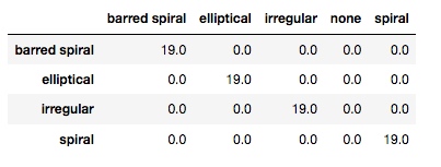
Figure 7: Confusion matrix given the training set as input.

The Jupyter notebook in HTML and IPYNB formats are available in S3.  One additional comment is needed.   Because this service is a black box, we have no idea what transfer learning service is use.

Microsoft Azure Cognitive Services Custom Vision.

The Microsoft Azure Custom Vison Service is another very well designed and easy to use system.   It is also a black box, so we have no idea how it works.  The assumption is that intended users don’t need to know and the designers are free to change the algorithm if they fine better ones.

Once you log in you create a new project as shown in Figure 8 below.   Then you can upload your training data using another panel in the interface.

Figure 8.   The  left panel defines the galaxy name and type.  The right panel is for uploading the training set.

Once the training set is in place you can see your project with a view of some of your images as shown in Figure 9.   There is a button to click to start the training.   In this case it takes less than a minute to see the results (Figure 10).

Figure 9.   The view of a sample of your training set.    The green button starts the training.

Figure 10.   The results from 2 iterations of the training.

If you are not pleased with the result of the training, you can try adding or removing images from the training set and train it again.

During the training with this data we made 3 iterations. the first was with the initial data. The system recognized that one of the elliptical galaxies was a duplicate, so the second iteration included an additional elliptical galaxy. The system will not allow a new iteration until you have modified the data, so the third iteration replaced a random spiral galaxy with another.  The results here are not great, but not bad for the small size of the training set.    As shown in Figure 11, the confusion matrix is better than the IBM case for distinguishing barred elliptical from elliptical but not as good at recognizing the irregular galaxies.

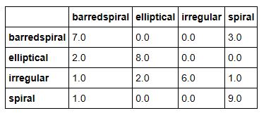
Figure 11.  Confusion matrix for Azure Custom Vision test.

Using the training data to compute the confusion we get an almost perfect score, but one barred spiral galaxy is recognized as spiral.

Figure 12.  Confusion Matrix for Azure Custom vison with training data

We looked at the case that confused the classifier and it can be seen to one that is on the border between barred spiral and spiral.   The image is contained in the full Jupyter notebook (html version,  ipynb version).

To use the notebook you need to have your prediction and training keys and the project id for the trained model.   You will also need to update your version of the Azure Python SDK.   The code below shows how to invoke the predictor.  The notebook gives the full details.

from azure.cognitiveservices.vision.customvision.prediction import prediction_endpoint
from azure.cognitiveservices.vision.customvision.training import training_api
training_key = 'aaab25your training key here 8a8b0' 
prediction_key = "09199your prediction key here b9ae" 
trainer = training_api.TrainingApi(training_key) 
project_id = 'fcbccf40-1bce-4bc4-b4ea-025d63f1014d' 
project = trainer.get_project(project_id)
iteration = trainer.get_iterations(project.id)[2]
image = “https://s3-us-west-2.amazonaws.com/learn-galaxies/bigtest/t5.jpg”
predictor = prediction_endpoint.PredictionEndpoint(prediction_key)
results = predictor.predict_image_url(project.id, iteration.id, url=image)
for prediction in results.predictions: 
  print("\t" + prediction.tag + ": {0:.2f}%".format(prediction.probability * 100)

The printed results give the name of each class and the probability that it fits the provided image.

Tensorflow transfer learning with Inception_v3

Google has built a nice package called Tensorflow For Poets that we will use for the next test.  This is part of their Google Developer Codelabs.

You need to clone the github repo with the command

git clone https://github.com/googlecodelabs/tensorflow-for-poets-2
cd tensorflow-for-poets-2

Next go to the subdirectory tf_files and create a new directory there called “galaxies” and put four subdirectories there: barredspiral, spiral, elliptical, irregular with each containing the corresponding training images. Next do

pip install --upgrade tensorflow

The Tensorflow code to do transfer learning and retrain a model is in the subdirectory scripts in a file retrain.py.   It follows the transfer learning method we described earlier by replacing the top to layers of the model with a new, smaller fully connected layer and a softmax layer.   We can’t go into the details here without a deep dive into Tenorflow code which is beyond the scope of this article.   Suffice it to say that it works very nicely.

The command to “retrain” the inception model is

python -m scripts.retrain \   
     --bottleneck_dir=tf_files/bottlenecks \   
     --how_many_training_steps=500 \   
     --model_dir=tf_files/models/ \   
     --summaries_dir=tf_files/training_summaries/"inception_v3" \   
     --output_graph=tf_files/retrained_graph.pb \   
     --output_labels=tf_files/retrained_labels.txt \   
     --architecture="inception_v3" \   
     --image_dir=tf_files/galaxies

If all goes well you will finally get the results that look like this

INFO:tensorflow:Final test accuracy = 88.9% (N=9)

Invoking the re-trained model is simple and you don’t need to know much Tensorflow to do it.  You essentially load the image as a tensor and load the model graph and invoke it with the input tensor.  The complete Python code for this in in the Jupyter notebook (in html and ipynb formats).

As with the other examples we have computed the confusion matrix for the test set and training set as shown below.

Figure 13.  Tensorflow test results.

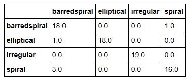
Figure 14.  Tensorflow results on the training set

As can be seen the retrained model as the usual difficulty distinguishing between spiral and barred spiral and irregular sometimes looks like elliptical and sometimes spiral.   Otherwise the results are not too bad.

Amazon SageMaker

SageMaker is a very different system from the tools described above.  This article will not attempt to cover SageMaker thoroughly and we will devote a more complete article to it soon.

Briefly, it consists of a complete system for training and hosting ML models.  There is a web portal but the primary user interface is Jupyter notebooks.   Figure 15 illustrate the view of the portal after we created several experiments.  It nicely illustrates the phases of SageMaker execution.

• You first create a Jupyter instance and a notebook. When you create a Jupyter notebook instance from the portal you are actually deploying a virtual machine on AWS.
• You use the notebook to create ML training jobs. The training jobs take place on a dynamically allocated container cluster.
• When training is complete you create a model which is stored and managed by SageMaker.
• When you have a model you can create an endpoint that can be used to invoke the model from your application.

Figure 15.  SageMaker portal interface.

To train a new model you provide the name of an AWS S3 bucket where your data is stored and a bucket where the output is going to be placed.

When the Jupyter VM spins up you see it in your browser.   The first thing you discover is a large collection of demo notebooks covering a host of topics.   You are not restricted to these.  There is also a library of tools to use Apache Spark from SageMaker.  You can also upload your own notebooks with TensorFlow or MXNet models for training.   Our you can create a docker image with your own algorithms.

In the example are interested here we discovered a SageMaker example notebook, Image-classification-transfer-learning.ipynb and made a copy we called sagemaker-galaxy-predict that you can access (in html or in ipynb  format).   As with the IBM and Microsoft examples, the actual transfer learning algorithm used is a black box, but there are some hints and parameters you can adjust.

When you train a deep neural network, you are find values for the millions of parameters in the network.  (As we have described above there are many fewer parameters in transfer learning.)  But there are an additional set of parameters, called hyperparameters, that describe the network architecture and the learning process.   In the case of the transfer learning notebook you must specify the following hyperparameters:  the number of layers in the network, the training minibatch size, the training rate and the number of training epochs.   There are defaults for these based on the example that SageMaker provides, but they did poorly for the galaxy experiment.    This left us with a four-dimensional hyperparameter space to explore.   After spending about two hours trying different combinations we came up with the table below.

# The algorithm supports multiple network depth (number of layers). They are 18, 34, 50, 101, 152 and 200
num_layers = 101
# we need to specify the input image shape for the training data
image_shape = "3,224,224"
# we also need to specify the number of training samples in the training set
num_training_samples = 19*4
# specify the number of output classes
num_classes = 5
# batch size for training
mini_batch_size =  21
# number of epochs
epochs = 5
# learning rate
learning_rate = 0.0018
top_k=2
# Since we are using transfer learning, we set use_pretrained_model to 1 so that weights can be 
# initialized with pre-trained weights
use_pretrained_model = 1

We are absolutely certain that these are far from optimal.   Once again we computed a confusion matrix for the test set and the training set and they are shown in Figure 16 and 17 below.

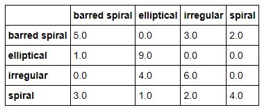
Figure 16.   Confusion matrix for SageMaker test data.

Figure 17.  Confusion matrix for SageMaker on training data.

As can be seen, these are not as good as our other three examples.    The failure is largely due to poor choices for the hyperparameters.  It should be noted that the Amazon team is just now starting a hyperparameter optimization project.   We will return to this example after that capability is available.

Conclusion

In this report we examined four computer vision transfer learning service.   We did this study using a very tiny example to see how well each service performed.   We used the simple confusion matrix to give us a qualitative picture of performance.  Indeed, these matrices showed us that distinguishing the barred spiral galaxies from the non-barred spiral ones was often challenging and that irregular galaxies are easy to misclassify.   If we want a quantitative evaluation we can compute the accuracy of each method using the test data.  The results are Azure = 0.75, Watson = 0.72, Tensoflow = 0.67 and SageMaker = 0.6.   However, given the very small size of the data sets, we argue that it is surprising that we could get reasonable results with such little effort.

Building the best galaxy classifier was not our goal here.  Real astronomers can do a much better job building systems that can answer much more interesting questions the classification task posed here. The goal of this project has been to show what you can do with cloud transfer learning tools.   The IBM and Azure tools were extremely easy to use and, within a few minutes you had a model constructed. It was not hard to access and use these models from a Python client.  The Tensorflow example from Google allowed us to do the transfer learning on a laptop.  SageMaker was fun to use (if you like Jupyter), but tuning the hyperparameters is a challenge.   A follow-up article will look at additional SageMaker capabilities.

Finally,  if any reader can improve on any of these results for this small dataset, please let me know!