
One of the most useful ways to uncover structure in high dimensional data is to project it down to a subspace, such as a 2-D plane, where hidden features may become visible. Of course, the challenge is to find the plane that best illuminates the structure. Manifold learning is based on the assumption that the system you are trying to model lies on or near a lower dimensional surface in the higher dimension coordinate space of the data. Picture the surface of a sphere or a curve in 3-D. If this manifold assumption about the data is true, it may be possible to “unfold’’ the surface so that a projection or other linear analysis makes the data easier to understand. Assume your data points are vectors in RN where N is big. If you are lucky and the data lies near a completely linear subspace of dimension k << N, then a truncated singular value decomposition (SVD) can be used to generate k eigenvectors that can be used to compactly encode the data. We have then reduced the N dimension analysis problem to one of dimension k.
In the case that the submanifold of the data is not linear, there are a dozen or so non-linear dimensionality reduction algorithms (Wikipedia has a good survery) and the ones discussed here are called autoencoders. At its most superficial level an autoencoder is a feed-forward neural network with a middle layer of much smaller dimension that the input and an output the same dimension as the input as shown in Figure 1.

Figure 1. A Basic Autoencoder network.
Let the dimension of the input vector be N and the dimension of the middle layer, which we call z, to be k. Represent the first half of the network by the function z = enc(x) and the second half the network be x’ = dec(z). An autoencoder network is trained to be the identity function. In other words, suppose we have m points xi, i=0,m-1, in RN, then we train the network so that xi’ = dec(enc(xi)) approximates xi for each i. The function enc(x) is our encoder function that maps RN to Rk , and the function dec(z) is the decoder that maps from Rk to RN. Of course, dec() and enc() are not unique and the depend on the way we train the network.
Before proceeding, it is worth noting the relationship between the autoencoder network and the truncated SVD. Let the matrix A of dimension m by N where the rows are our vectors xi i=1..m. The SVD decomposition of A is given by A = UVW where U is m by m, V is a diagonal matrix of size m by N and W is a N by N matrix. U and V have the property that UTU = I, where UT is the transpose of U and WWT = I. The values on the diagonal of V are the singular values of A in decreasing size. Multiplying A=UVW on the right by WTW yields the equation AWTW = UVWWTW = UVW = A. Another way of saying this is if x is a row of A, then x = (xWT)W. Pick the k largest singular values and define A’ = UkVkWk where Uk is the first k columns of U and Wk are the first k rows of W and Vk is our k by k matrix of top eigenvalues. In these terms, zi = xi WTk is the encoding of xi into RK and xi’ = ziWk corresponds to the decoder function. In fact, if the neural net for the autoencoder is linear and only one layer these two concepts are identical. In other words, the truncated SVD is a degenerate form of a neural network autoencoder.
This is nicely illustrated in the paper by Baldi et. al. in the paper “Deep Autoencoder Neural Networks for Gene Ontology Annotation Predictions”. In their case the m vectors X correspond to genes and the components (columns of A) correspond to gene annotations. By choosing the right eigenvalues for Zk and the right value of k, the terms of A’ are good predictors of gene annotations. Of course, the point of the paper is to demonstrate that that a well-trained non-linear autoencoder is an even better predictor and they demonstrate that nicely.
Great examples from LBNL
Recently, a lovely blog article A look at deep learning for science by Prabhat gave us an excellent overview of some uses of deep learning technology in science applications and several of these were applications of autoencoders. We will take a brief look one these and then take a deeper look at autoencoders and illustrate them with simple example.
One nice example from Prabhat’s blog is an experiment to classify the events generated by the Daya Bay Neutrino Experiment. In the blog, Samuel Kohn, Evan Racah, Craig Tull, Wahid Bhimji discuss the challenge of identifying events that are mixed with noise in their search for antineutrino interactions. The noise comes from external cosmic ray and other sources. In a related paper , “Revealing Fundamental Physics from the Daya Bay Neutrino Experiment using Deep Neural Networks” Racah, et. al. describe the results of using a deep convolutional network trained with labeled events to recognize the various types of signal. In the blog post they describe the use of an denoising convolutional autoencoder to understand how features of the antineutrino events differ from the noise.
A denoising autoencoder is one where the input to the encoder is a corrupted version of the image. So the training of the autoencoder is pushing it to recover the original image from the corrupted one. In the Daya Bay example, the trained denoising autoencoder was nicely able to separate the noise signals from the good ones.
The way they demonstrate the separation is to use another dimensional reduction tool, t-distributed stochastic neighbor embedding (t-SNE) that can take the set of images of the data in the encoded space and reduce it to a 2-D image. This is a very nice statistical method of dimensional projection. It works by build a distribution pij of pairs in the high dimensional space. Then it tries to create a 2-D distribution qij of points that has a similar distribution. To do that it uses the Kullback-Leibler divergence
KL(p||q) = Ʃij(pij log (pij/qij) )
The KL divergence measures now many extra bits (or ‘nats’) are needed to convert an optimal code for distribution P into an optimal code for distribution Q. (We mention this because we will use it again below.)
Variational Autoencoders
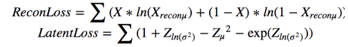
A variational autoencoder (VAE) is one that is based on creating an encoding that has a probabilistic distribution that generates a good model of the input data from some system. In a VAE, one views our encoding vector z as a latent variable with a probability density function P(z) such that if we sample z from P(z) we have a high probability that the decoded vector d(z) is a good example from or very near the manifold for our data X. Given this density function we can model the system that generated X in two way. First, we now have a way to pick values from the distribution that generate new potential samples of our system. Second, we can take a candidate x as a possible member of the system, we can then use the computed P(enc(x)) as probabilistic evidence that the candidate is a likely member. The architecture of the VAE is similar to the standard with one major exception. Rather than generate an explicit vector in the imbedding space we generate a Gaussian density function defined by a mean and a standard deviation (actually the log of the squared standard deviation which is assumed to be diagonal) for each of our sample points. We then sample from this distribution and generate a value for Z which can be input to the decoder. This is illustrated in the following diagram and equations below.
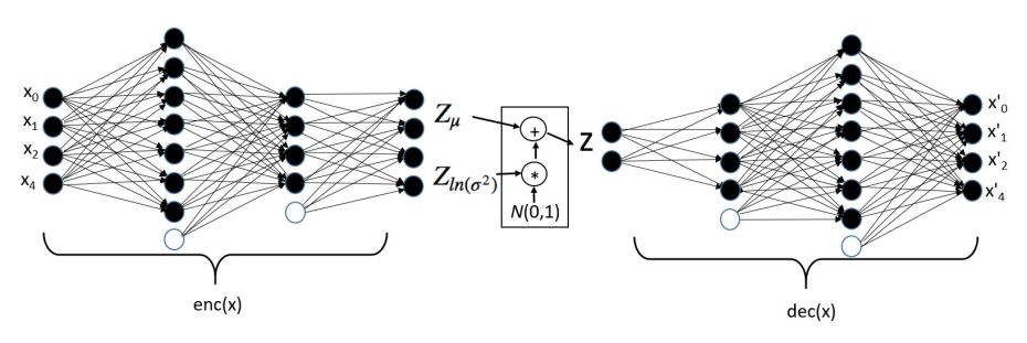
Figure 2. Variational Autoencoder architecture.
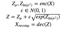
Figure 3. VAE equations.
Training for the VAE also differs from that of the denoising AE. We want dec(enc(xi )) to be as near to xi as possible, but we also want to make sure the distribution of the latent variable P(Z) to be appropriate for the input model manifold. To train the network to behave according to this plan we need a carefully designed optimization plan. We also need some more notation. We borrow it from a nice blog by Jaan Altosaar. Let the encoder be a parameterized distribution qϴ(z|x) and the decoder be pФ(x|z). We want the information loss from the across the whole network to be as small as possible for each data point Xi. To do that we want to minimize −Ez∼qθ(z∣xi)[logpϕ(xi ∣ z)]. However, we also want to make sure that the distribution difference between then encoder distribution qϴ(z|x) and p(z), the Gaussian distribution we desire for z. To do this we use the Kullback-Leibler divergence described above. The result is a loss function
li(θ,ϕ)=−Ez∼qθ(z∣xi)[logpϕ(xi∣z)] + KL(qθ(z∣xi) ∣∣ p(z))
To demonstrate how this works for a real example, we could use the standard example of hand written digits, but that has been done often before. Instead we will take a python script for a variational autoencoder in Tensorflow originally designed by Jan Hendrik Metzen for MNIST and show how to modify it and train it for a different data set. The Jupyter notebook that generates the code for this example available as an html file and an ipynb file. In modifing Metzen’s code we will commit one serious statistical crime which we will explain later, but the results are still interesting.
The data we will use comes to us courtesy of Maryana Alegro from the University of California, San Francisco. It is really interesting. Dr. Alegro tells us that the data consists of “images of neurons drawn from real immunofluorescence (IF) microscopy of post-mortem human brain tissue. These are part of an UCSF study that aims to understand Alzheimer’s disease (AD) development in brain stem nuclei, which are affected by the disease years before initial symptoms onset. The red cells are stained using a fluorescence marker called CP-13 that binds to TAU tangles, commonly associated with AD. Green cells are stained for aCasp-6, which binds to proteins present during apoptosis (cell death) and yellow cells that have overlap of both markers.” The goal for their project is to was quantifying the presence of these three classes in IF images can help understand if the presence of TAU is really causing cell death in brain stem nuclei. They have a very nice paper “Automating cell detection and classification in human brain fluorescent microscopy images using dictionary learning and sparse coding” in Journal of Neuroscience Methods 282 (2017) 20–33, that describes some of their work. The figure below illustrates the three classes of cell images.

Figure 4. Example images of class 0, 1 and 2 from left to right.
The link to download the data is here.
In the demonstration that follows very little information is shed on the UCSF scientific challenge, but we are able to use this data set to easily build a classifier based on Gradient Boosting from Scikit-learn. This was accomplished by reducing the data to 28 by 28 24-bit RGB images. Also because there is a very small number of class 0 images in relation to the others, we duplicated half of them in the data set to bring them up to parity for training. With a total of 1032 images (including the duplicates), the classifier did reasonably well. The confusion matrix is shown below when tested on 200 images held back from the training.
| class 0 | class 1 | class 2 | |
| class 0 | 96.88% | 0 | 3.13% |
| class 1 | 4.00% | 88.00% | 8.00% |
| class 2 | 13.11% | 6.56% | 80.33% |
Figure 5. Image classification confusion matrix for Gradient Boosting. (Class 0 numbers are not accurate because of duplicate images in the test set that are also in the training set.)
We now consider how well we can model the image space using a variational autoencoder. The images have been transform into vectors real numbers of length 28*28*3. Each value is in the range [0, 1]. While this does not classify as a truly Bernoulli distribution we will treat it as such. The color spike for each class is “similar” to a Bernoulli distribution (this is the statistical crime we referred to earlier). We need this because the Python VAE we are using is from Metzen assumes the decoder induces a Bernoulli distribution on the image space. This allows him to translate the li(θ,ϕ) expression above into the optimization involving a reconstruction loss term plus a simple for for the Kullback-Leibler divergence KL(qθ(z∣xi) ∣∣ p(z)) with ϴ = (Zµ, ZΣ) as the latent loss.
The objective function is –ReconLoss – 0.5*LatentLoss. The modified version of the VAE code is in Notebook VAE. After training for 1500 epochs it is useful look at the quality of the reconstructions. This is illustrated in Figure 6 below. There are two things to know. The Python computer vision library that we used to convert the original jpg images into the normalized vectors also changed the apparent colors when displayed. So vivid red cells and yellow cells now appear as shades of blues. Also the picture shows a reconstruction based on a random sample near Zµ as shown in Figure 2 and 3. So these are “nearby” reconstructions from the model manifold.
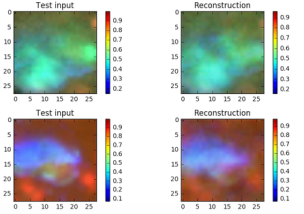
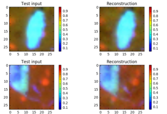
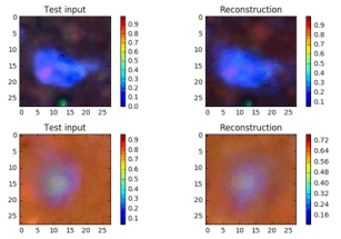

Figure 6. Sample images and a sample reconstruction
Once the network has been trained we can sample from the latent space Z and generate images from the model.
One simple test we can make is to see reconstructions of a given class can be recognized by our classifier as belonging to the correct class. We generated 100 reconstructions from each of the three classes and presented them to the trained gradient boosting classifier described above. The results are given in the confusion matrix below.
| class 0 | class 1 | class 2 | |
| class 0 | 76% | 9% | 17% |
| class 1 | 4% | 92% | 4% |
| class 2 | 11% | 9% | 80% |
As you can see, class 0 and class 2 tend to be confused but not much more than with the original training data.
Another interesting exercise is to select 5 of our samples xi i=1..5 in one of the classes and then compute a path connecting the encoded image of enc(xi) and enc(xi+1) with line segments in the latent space and then compute the reconstruction for each point on the path.. By taking 100 samples for each lin segment we generate a total of 500 “candidate” cells from our model. From that we can make a movie. It is shown below. it is interesting to note that the path largely follows the model manifold, but it often clearly drifts off generating unlikely images.

Figure 7. A movie following a “loop” on the model manifold in latent “z” space decoded to image space.
One last thing we can do with this little example is to look at the t-SNE projection of enc(xi) in the latent space which is of dimension 20. This projection is shown below in Figure 8.
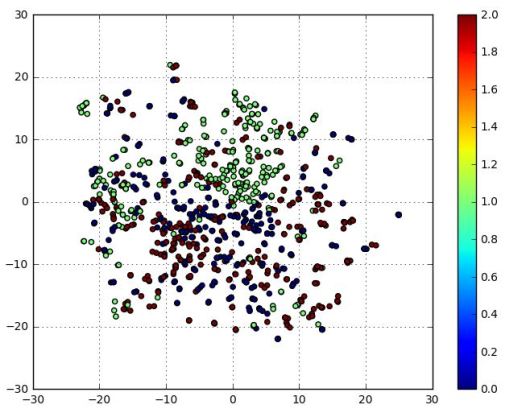
Figure 8. T-SNE projection of the latent space image of the cell images.
As you can see the class1 (green) cells are reasonably well clustered, but the class0 (blue) and class2 (red) cell images not as well separated. This is consistent with the confusion matrix results.
This example is based on a very tiny data collection and there are no substantial scientific conclusions that we can come to regarding the original scientific goals of the UCSF project. However, we have demonstrated that we can make a model of the image data manifold that can generate samples that are believable. A much better illustration of this idea is described next.
Galaxy Models
In Prabhat’s blog post, Jeffrey Regier and Jon McAullife describe the use of a variational autoencoder to model galaxies. More specifically they want a probabilistic model of images that assigns high probability to images of galaxies. In their paper with Prabhat “A deep generative model for astronomical images of galaxies”, they describe their VAE and a detailed derivation analysis. They trained the VAE on 43,444 69-by-69 pixel images of galaxies from the Sloan Digital Sky survey. In 97% of the cases in test set they were able to assign higher probabilities of correct identification than the best previous model.
Cosmology Models
Debbie Bard, Shiwangi Singh and Mayur Mudigonda have been investigating cosmological mass maps. These maps are very important for identifying interesting configurations of galaxies that can create phenomena such as gravitational lensing that can help us understand dark matter. Another very interesting application of autoencoders is to use them to identify important features of various simulated cosmologies so that they can be compared those same features in real observed mass maps. In this case they used denoising autoencoders (trained with 5000 simulated maps) they were able to classify the model that produced the best data 80% of the time.
There are several other excellent examples in Prabhat’s blog and we strongly recommend reading it. Clearly science represents an area where deep learning can be a great tool for modeling nature. There are still many challenges but the progress being made suggests that this is a green field for research.
