In this note we provide a simple illustration of how the ‘classic’ deep learning tool LSTM can be used to model the  solution to time dependent differential equations.  We begin with an amazingly simple case: computing the trajectory of a projectile launched into the air,  encountering wind resistance as it flies and returns to earth.  Given a single sample trajectory, the network can demonstrate very realistic behavior for a variety of initial conditions. The second case is the double pendulum which is well known to generate chaotic behavior for certain initial conditions.   We show that a LSTM can effectively model the pendulum in the space of initial conditions up until it encounters the chaotic regions.

Using Neural Nets to Generate Streams of Data

Much of the recent excitement in deep learning has come from the ability of very large language models (such as gpt-3 from OpenAI) to generate streams of text to solve impressive tasks such as document summarization, writing poetry, engaging in dialog and even generating computer code.      In the case of scientific application, deep learning models have been used to tackle a number of interesting forecasting challenges.  

There are two major differences between natural language processing and physical system modeling.  First, natural language has a finite vocabulary and the model must include an embedding that maps words into vectors and a decoder  that maps the neural network outputs into a probability distribution over the vocabulary.   In the case of physical systems, the data often consists of  streams of vectors of real numbers and the embedding mapping may not be needed.  The second difference is that physical systems can often be modeled by differential equations derived from the laws of physics.   There are often strong parallels between the formulation of the differential equation and the structure of the neural network.   We examined this topic in a previous article where we described the work on Physically Inspired Neural Networks and Neural Ordinary Differential Equations.   Solving a time dependent differential equation is often stated as an initial value problem:  Given the equations and a consistent set of k critical variables at some time t₀, a solution is an operator D that defines a trajectory through R^k that satisfies the equations.

Unless a differential equation has a known, closed form solution, the standard approach is numerical integration. We can describe this as an operator Integrate which takes vector of  initial variable values at t₀ ,V₀ in R^k  Integrate( V₀)  to a sequence V_i in R^k 

so that the appropriate finite difference operations when applied to the sequence of V_i approximately satisfy the differential equations. The Integrate operator is normally based on a carefully crafted numerical differential equation solver and   the number of time steps (T_n) required to advance the solution to a desired end configuration may be very large and the computation may be very costly.   Alternatively, the Integrate operator may be based on a pretrained neural network which may be as accurate and easier to compute.   We are now seeing excellent examples of this idea.

Rajat Sen, Hsiang-Fu Yu, and Inderjit Dhillon consider the problem of forecasting involving large numbers of time series.  By using a clever matrix factorization they extract a basis set of vectors that can be used with a temporal convolutional network to solve some very large forecasting problems.  JCS Kadupitiya, Geoffrey C. Fox, and Vikram Jadhao consider classical molecular dynamics problems and they show that an integrator based on Long Short Term Memory (LSTMs) can solve the Newton differential equations of motion with time-steps that are well beyond what a standard integrator can accomplish.   J. Quetzalcóatl Toledo-Marín, Geoffrey Fox, James Sluka and James A. Glazier  describe how a convolutional neural network can be used as a “surrogate” for solving diffusion equations. 

In his draft “Deep Learning for Spatial Time Series”,  Geoffrey Fox generalizes the LSTM based differential equation integrators described above (and in our examples below) to the case of spatial as well as temporal time series.   To do this he shows how to integrate the encoder of a Transformer with and LSTM decoder.   We will return to the discussion of Fox’s report at the end of this post.

There are many variations of neural networks we could use to approach the problem of forecasting streaming data.   Transformers are the state-of-the-art for NLP, having totally eclipsed recurrent neural nets like the Long Short-term Memory (LSTM).   When put to the task of generating sentences LSTM tend to lose context very quickly and the results are disappointing.  However, as we shall see, in the case of real data streams that obey an underlying differential equation they can do very well in cases where the solutions are non-chaotic.   We will look at two  very simple  examples to illustrate these points

Case1.  The Trajectory of a Ball Thrown Encountering Wind Resistance.

Consider the path of a ball thrown with initial speed v and at an elevation angle θ.  As it flies it encounters a constant drag and eventually falls back to earth.  With the initial position as the origin, the differential equation that governs the path of our ball is given by  

where g is the gravitational acceleration and u is the drag caused by the air resistance as illustrated in the figure  below.

Figure 1.   The path of our ball given initial speed v and elevation angle θ

Wikipedia provides a derivation of these equations and a Python program that generates the numerical solution illustrated above.   We will use a modified version of that program here.   A standard ordinary differential equation solver (odeint) can be used to generate the path of the ball. 

We will use a simple LSTM network to learn to reproduce these solution.  The network will be trained so that if it is given 10 consecutive trajectory points (x_i,y_i) for i in [0,9] it will generate the next point (x₁₀,y₁₀).   To make the LSTM generate a path for a given value of v and θ we provide the first 10 points of the solution and then allow the LSTM to generate the next 100 points.

 We will use the most trivial form of a LSTM as shown below to define our model.

The differential equation requires 4 variables (x, y, v_x, v_y)  to make a well posed initial condition,  however our model has an input that is only two dimensional.  To provide the velocity vector we give it a sequence of 10  (x,y) pairs, so our model is

The way the model is trained is that we take a trajectory computed by the ODE Solver computed by the projectile_motion function and break that into segments of length 11.   The LSTM is given the first 10 pairs of points and it is trained to predict the 11^th point.  This is a training set of size 100.  (The details of the training are in the Jupyter Notebook in the github repo for this article.  )

We have a simple function makeX(angle, speed) that will compute the ODE solution and time to ground.  The training set was generated with the path p = makeX(30, 500).   A second function  OneStep(path) that takes a computed path and uses the first 10 steps to start the model which goes until it reaches the ground.  OneStep (less a plotting component and the ground hitting computation) is shown below.   The data is first normalized to fit in the (-1, 1) range that neural net expects.  We then take the first 10 elements to start a loop which predicts the 11^th step.  That is appended to the list and we continue to predict the next step until done. 

  If we run OneStep with the path from the training data it is a perfect fit.  This, of course is not surprising. However if we give it a different initial angle or different initial speed the network does an very good job on a range of initial conditions.  This is illustrated in Figures 2 and 3 below.

Figure 2.  Comparing the ODE solver to the LSTM for a fixed speed and a range of angles.

Figure 3.   Comparing the ODE solver to the LSTM for a fixed angle and a range of speeds.

The further we move from our initial training path, the less accurate the result.  This is shown in Figure 4.

Figure 4.   angle = 10, speed = 500.  The LSTM overshoots slightly but ends correctly.

We also trained the network on 4 different paths.  This improved the results slightly.

Case 2. The Double Pendulum

The double pendulum is another fascinating case with some interesting properties.  It consists of two pendulums, with the second suspended from the end of the first.  As shown in figure 5, it can be characterized by two angles θ₁ and θ₂ that measure the displacements from vertical, the length of the two pendulum arms L₁ and L₂ and the masses M₁ and M₂. 

Figure 5.  The double pendulum

The equations of motion are in terms of the angles, the angular velocities and the accelerations.  The

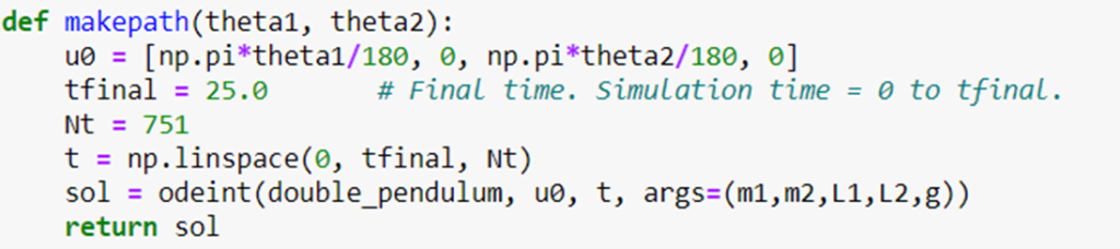
We have adapted a very nice program by Mohammad Asif Zaman (github) by adding our LSTM network as above.   The initial condition is to hold the configure vector in a position for a given value for the two angles with the angular velocities both zero and release it.   We have a function
double_pendulum(V,t,m1,m2,L1,L2,g) that evaluates the differential equations given the configuration and we use the standard ODE solvers to integrate the solution forward from the initial configuration with

Using different values for parameters for d1 and d2 we can generate a variety of behaviors including some that are very chaotic. 

Our LSTM network is as before except its initial and final dimension is 4 rather than 2.  We train this as before but integrate much farther into the future.   (Again, the details are in the notebooks in github.)

We have created a version of the OneStep function that allows us to see the trajectories.  It is more interesting to look at the trajectory of the lower mass.   In Figure 6 below we see on the right the positions of the double pendulum with the initial condition angles θ₁= -60 degrees and θ₂ = 60 degrees.   We then show the configurations at T = 20 and T = 80.

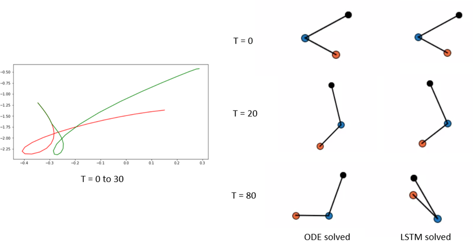
Figure 6.   Double Pendulum.   On the left is the path of the ODE solution in red and the LSTM solution in green.

By looking at the path traces on the left the two solutions for this configuration diverge rapidly.   Using smaller angles we get much more stable solutions.   Below is the trace for θ₁= -20 degrees and θ₂ = 35 degrees.

Figure 7.  Blue mark is starting point, yellow is when the two solutions begin to diverge.

Below we have the animated versions of the ODEsoltion and the LSTMsolution for this case. Below that in Figure 9 is the illustration of the chaotic case (-50, 140)

• 

• 

Figure 8 Left is ODE solution for -20 degrees, 35 degrees. Right is LSTM solution

Figure 9. Left is chaotic ODEsoltion for -50 degrees, 140 degrees. Right is failed LSTMsolution

Conclusions

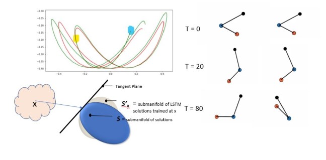
The experiment described here used only the most trivial LSTM network and tiny training set sizes.   The initial value problems we considered were a two dimensional submanifold of the 4 dimensional space:  in the case of the projectile, the origin was fixed and the speed and angle were free variables and in the pendulum, we had the two angles free and the initial angular velocities were set to 0.  Each point of the initial conditions is a point on the configuration manifold (which is a cylinder defined by angle and speed for the projectile and a torus defined by the two angles of the pendulum).  The differential equations specify a unique path from that initial point along the configuration manifold.  The LSTM defines another path from the same initial point along the manifold.  The question is  how are these two paths related?

We noticed that training the LSTM with one solution allowed the LSTM to generate reasonably good solutions starting from points “near” the training initial value point.   It is interesting to ask about the topology of set of solutions S to the differential equations, in the region containing the solution generated by an initial value point x.   Consider the case of the projectile when the wind resistance is zero.  In this case the solutions are all parabolas with a second derivative that is -g.   This implies that any two solutions differ by a function that has a second derivative that is zero: hence they differ by a simple line.  In this case he topology of S is completely flat.   If the wind resistance is non-zero, the non-linearity of the equations tells us that the submanifold S is not completely flat.   If we consider the submanifold of solutions S’_x for the LSTM trained on the single initial value point x, we noticed that values near x generated solutions in S’_x that were very close to the solutions in S near those generated  by points near x.  We suspect that the two submanifolds S and S’_x share the same tangent plane at x.   We attempted to illustrate this in Figure 9 below.

Figure 9.  Depiction of the tangent planes to two submanifolds that have the same solution for a given initial condition x.

In the case of the double pendulum,  the  shape of S is much more complex.  The LSTM manifold is a good approximation of the pendulum in the stable region, but once a starting point is found at the edge of the chaotic region the LSTM solution fall apart. 

In his draft ”Deep Learning for Spatial Time Series”, Fox shows a very general and more sophisticated application of neural networks to time series.   In particular, he addresses sequences that are not limited to time series as we have discussed here.  He describes a concept he calls a “spatial” bag which refers to a space-time grid of cells with some number of series values in each cell.  For example, cells may be locations where rainfall, runoff and other measures are collected over a period of time.   So location in the spatial bag is one axis and time is the other.   Making prediction along the spatial direction is  analogous to sequence to sequence transforms  and prediction along the time axis is similar to what we have described here.  The network his team used is hybrid with a Transformer as encoder and LSTM as a decoder.   Because the bag is an array of discrete cells,  the Transformer is a natural choice because the attention mechanism can draw out the important correlations between cells.  The LSTM decoder can generate streams of output in a manner similar to what we have done.   The paper shows convincing results for hydrology applications as well as COVID-19 studies.   I expect much more to come from this work.