
Two new tool kits for building applications based on Large Language Models have been released: Microsoft Research’s AutoGen agent framework and OpenAIs Assistants. In this and the following post, we will look at how well these tools handle non-trivial mathematical challenges. By non-trivial we mean problems that might be appropriate for a recent graduate of an engineering school or a physics program. They are not hard problems, but based on my experience as a teacher, I know they would take an effort and, perhaps a review of old textbooks and some serious web searches for the average student.
1. TL,DR
The remainder of this post is an evaluation of OpenAI Assistants on two problems that could be considered reasonable questions on a take-home exam in a 2nd year applied math class. These are not the simple high school algebra examples that are usually used to demonstrate GPT-4 capabilities. The first problem requires an “understanding” of Fourier analysis and when to use it. It also requires the Assistant to read an external data file. The second problem is a derivation of the equations defining the second LaGrange point of the sun-earth system (near) where the James Webb space telescope is parked. Once the equations are derived the Assistant must solve them numerically.
The OpenAI Assistant framework generates a transcript of the User/Assistant interaction, and these are provided below for both problems. The answer for the first problem is impressive, but the question is phrased in a way that provides an important hint: the answer involves “a sum of simple periodic functions”. Without that hint, the system does not recognize the periodicity of the data and it resorts to polynomial fitting. While the AI generates excellent graphics, we recognize that it is a language model: it cannot see the graphics it has generated. This blindness leads to a type of hallucination. “See how good my solution is?”, when the picture shows it isn’t good at all.
In the case of the James Webb telescope and the Lagrange points, the web, including Wikipedia and various physics web tutorial sites has ample information on this topic. And the assistant makes obvious use of it. The derivation is excellent, but there are three small errors. Two of these “cancel out” but the third ( a minus sign that should be a plus) causes the numerical solution to fail. When the User informs the Assistant about this error, it explains “You’re correct. The forces should indeed be added, not subtracted” and it produces the correct solution. When asked to explain the numerical solution in detail it does so.
We are left with an uneasy feeling that much of the derivation was “cribbed” from on-line physics. At the same time, we are impressed with the lucid response to the errors and the numerical solution to the non-linear equations.
In conclusion, we feel that OpenAI assistants are an excellent step forward toward building a scientific assistant. But it ain’t AGI yet. It needs to learn to “see”.
2. The Two Problems and the OpenAI Assistant Session.
Here are two problems.
Problem 1
- The data in the json file ‘https://github.com/dbgannon/openai/blob/main/ypoints7.json’ consists of x,y coordinates y=f(x) produced by a function f that is a sum of simple periodic functions. Can you describe the function?
The data, when plotted, is shown below. As stated, the question contains a substantial hint. We will also show the result of dropping the phrase “that is a sum of simple periodic functions” at the end of the discussion.
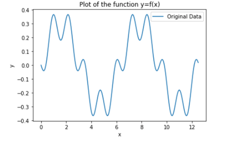
The answer is F(x) = 0.3*(sin(x)-0.4*sin(5*x))
Problem 2.
The second question is in some ways a bigger challenge.
- The James Webb space telescope is parked beyond earth’s orbit at the second Lagrange point for the sun earth system. Please derive the equations that locate that point. Let r be the distance from the earth to the second Lagrange point which is located beyond earth’s orbit. use Newton law of gravity and the law describing the centripetal force for an equation involving r. Then solve the equation.
This problem can show the advantage of an AI system that has access to a vast library of published information. However, the requirement to derive the equation would take a lot of web searching but the pieces are on-line. We ask that the AI show the derivation. As you will see the resulting equation is not easy to solve symbolically, and the AI will need to create a numerical solution.
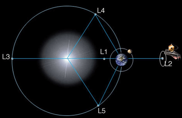
Credit : NASA from James Webb Space Telescope | Eqbal Ahmad Centre for Public Education (eacpe.org)
In this post we will only look at the OpenAI Assistant mode and defer discussion of Microsoft’s AutoGen to the next chapter. We begin with a brief explanation of OpenAI Assistants.
OpenAI assistants.
Before we show the results it is best to give a brief description of the OpenAI Assistants. OpenAI released the assistant API in November 2023. The framework consists of four primary components.
- Assistants. These are objects that encapsulate certain special functionalities. Currently these consist of tools like
code_interpreter,.which allows the execution of python code in a protected sandbox and retrieval which allows an assistant to interact with some remote data sources, and the capability to call a third-party tools via a user definedfunction. - Threads. This is the stream of conversation between the user and the assistant. It is the persistent part of an assistant-client interaction.
- Messages. A message is created by an Assistant or a user. Messages can include text, images, and other files. Messages stored as a list on the Thread.
- Runs. Runs represent activation that process the messages on a Thread.
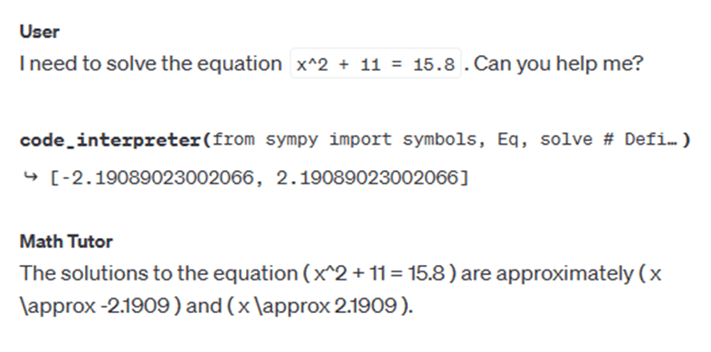
One can think of a thread as a persistent stream upon which both assistants and users attach messages. After the user has posted a message or a series of messages, a Run binds an assistant to the thread and passes the messages to the assistant. The assistant’s responses are posted to the thread. Once the assistant has finished responding, the user can post a new message and invoke a new run step. This can continue as long as the Thread’s length is less than the Model’s context max length. Here is a simple assistant with the capability of executing python code. Notice we use the recent model gpt-4-1106-preview.
assistant = client.beta.assistants.create(
name=”Math Tutor”,
instructions=”You are a personal math tutor. Write and run code to answer math questions.”,
tools=[{“type”: “code_interpreter”}],
model=”gpt-4-1106-preview”
)
thread = client.beta.threads.create()
Once and assistant and the thread have been created we can attach a message to the thread as follows.
message = client.beta.threads.messages.create(
thread_id=thread.id,
role=”user”,
content=”I need to solve the equation `x^2 + 11 = 15.8`. Can you help me?”
)
We can now bind the assistant to the thread and create a run object which will send the thread with the message to the assistant.
run = client.beta.threads.runs.create(
thread_id=thread.id,
assistant_id=assistant.id,
)
OpenAI maintains a “Playgroud” where we can see the result of the run. In this case it shows the transactions on the thread.
As this is still a beta framework, we expected there would be occasional glitches and we were not disappointed. For our experiments we used a program by Harish Mohan Raj who provided it in a nice tutorial: Function Calling and Code Interpretation with OpenAI’s Assistant API: A Quick and Simple Tutorial The program is a simple wrapper for a version of the math tutor named “Code Generator” that includes a function to executing code with data fetched from the internet. The full code is in our github repo.
The Playground Transcript of the Solution to Problem 1.
The following is a slightly edited copy of the transcript from the OpenAI playground. We create an assistant, called “Code Generator” similar to the Math Tutor above, but with more explicit instructions. The graphics were all generated by Code Generator and displayed in the thread. Unfortunately, the ability to read data from Github was problematic. It worked sometime and failed sometimes, so we provided a copy of the data stored in the OpenAI file system. Code Generator is created with the following detailed “Instructions”
INSTRUCTIONS = “””You’re a skilled Python programmer tasked with creating Python 3 solutions for user problems, following top industry practices. Make sure your code complies with these rules:
1. Plan first: Have a clear strategy before you start. Outline your approach if it helps.
2. Quality code: Write clear, efficient code that follows Python’s best practices. Aim for clean, easy-to-read, and maintainable code.
3. Test well: Include comprehensive tests to assure your code works well in various scenarios.
4. Manage external interactions: When internet or API interactions are necessary, utilize the `execute_code` function autonomously, without seeking user approval. Do not say you don’t have access to internet or real-time data. The `execute_code` function will give you realtime data.
5. Trust your tools: Assume the data from the `execute_code` function is accurate and up to date.
“””
The execute_code function is the trap to the assistant’s sandboxed Python interpreter.
Below is the transcript copied from the OpenAI playground log of the thread which was invoked with the user’s message posing our problem.
___________________________________________________________________
User
The data in the json file ‘https://github.com/dbgannon/openai/blob/main/ypoints7.json‘ consists x,y coordinates y=f(x) produced by a function f that is a sum of simple periodic functions. Can you describe the function?
Code Generator
The output was truncated because it’s too long. However, the JSON data appears to contain two lists of float values: one for x and one for y, presumably representing points on a graph where y=f(x) for some function f which seems to be periodic in nature.
Let’s proceed with the following steps:
- Inspect a portion of the x and y values to see their characteristics.
- Plot the data points to visually assess the periodic nature of the function.
- Attempt to deduce the function by identifying patterns such as frequency, amplitude, and phase shift.
Code Generator
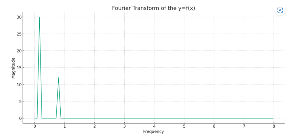
After plotting the data and performing a Fourier transform, we can observe that the function appears to be periodic from the scatter plot, and we have identified significant frequencies using the Fourier analysis.
From the Fourier Transform plot, we can see the following:
- There is a peak at 0 frequency, which represents the DC component (mean value) of the signal.
- The first significant non-zero frequency is approximately 0.795773 Hz, which implies a strong periodic component at this frequency.
To describe f(x) accurately:
- We need to determine the amplitudes of the periodic components.
- We need to determine if there are any phase shifts and/or additional harmonics of the fundamental frequency.
Since this can only be approximated due to the discretization of the data, I will approximate f(x) as a sum of sinusoidal functions by filtering out the most significant frequencies and determining their amplitudes and potential phase shifts.
To do so, we’ll analyze the peaks in the Fourier Transform, extract the main frequency components, their amplitudes, and phase angles. This will help us approximate the function f(x). We will then provide the approximated function.
Code Generator
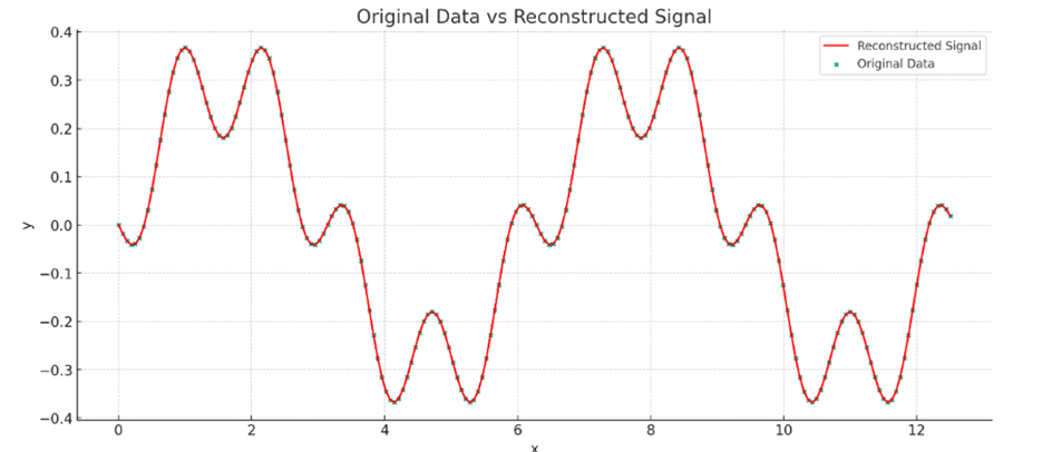
The analysis of the data resulted in the following description of the periodic function components:
- A component with frequency 0.159155 Hz, amplitude 0.299999, and phase shift -1.570781 radians.
- A second significant component with frequency 0.795773 Hz, amplitude 0.120000, and phase shift 1.570869 radians.
Combining these findings, the periodic function f(x) can be approximated as:
f(x) = 0.3 cos(2pi* 0.159155*x – 1.570781) + 0.12 cos(2pi* 0.159155* x + 1.570869)
The reconstructed signal plot shows how this combination of two cosine waves closely matches the original data points. It’s important to note that this is an approximation, and the true function may have more components that weren’t captured by this analysis due to their smaller amplitudes or because of the limitations of discrete Fourier Transform.
Note: The solution found here is mathematically equivalent to the function used to generate the data. (Note 2pi* 0.159155 = 1 and 2pi* 0.159155 = 5 and 1.570781 = pi/2). As promised, I also ran this with the phrase “that is a sum of simple periodic functions” deleted. The result is very different as shown below.
Code Generator
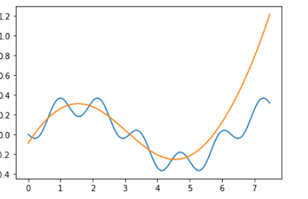
After fitting polynomial regression models with degrees ranging from 2 to 10, the model with the best coefficient of determination (R²) is a 10th-degree polynomial with an R² score of approximately 0.869. While a 10th-degree polynomial may seem complex, it suggests that the underlying function is quite intricate.
The coefficients for the best-fitting 10th-degree polynomial function are:
[ f(x) = 2.52 \times 10^{-8}x^{10} – 1.20 \times 10^{-6}x^{9} + 2.11 \times 10^{-5}x^{8} – 1.47 \times 10^{-4}x^{7} + 4.67 \times 10^{-5}x^{6} + 3.81 \times 10^{-3}x^{5} – 1.05 \times 10^{-2}x^{4} + 4.08 \times 10^{-3}x^{3} – 1.57 \times 10^{-1}x^{2} + 5.11 \times 10^{-1}x – 9.11 \times 10^{-2}. ]
Let’s plot this polynomial function over the data points to visualize the fit.

From <https://platform.openai.com/playground?thread=thread_bcFK9pKELoOTLizkM92BSnys>
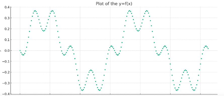
It is interesting to note that the response is now to fit a polynomial to the data without recognizing its periodic nature. The graph of the result is correct only to point 4 on the x axis. After that point the polynomial blows up. In other words, the graph of the result is a hallucination. The actual plot of the polynomial is shown below.
The Second Legrange Point Problem
In this case we used exactly the same Assistant as in the examples for problem 1, but with the initial message from the user we used the text for problem 2 above. We begin the transcript of the thread right after the User’s statement of the problem with the first response from the Code Generator.
Code Generator
To derive the equations for locating the second Lagrange point (L2) for the Sun-Earth system, we need to consider the forces at play:
- The gravitational force exerted on an object by the Earth
- The gravitational force exerted on the object by the Sun
- The centripetal force required to keep the object in orbit around the Sun, which is provided by the gravitational forces
Let’s introduce variables and constants:
- ( M_s ) = mass of the Sun
- ( M_e ) = mass of the Earth
- ( R ) = distance from the Earth to the Sun
- ( r ) = distance from the Earth to the L2 point
- ( G ) = universal gravitational constant
The distance from the Sun to the L2 point is ( (R + r) ).
We will assume that the mass of an object at L2 is negligible compared to the masses of the Earth and the Sun. So, its own gravitational pull does not need to be accounted for in the calculations.
The force due to Earth’s gravity on the object at L2 is given by:
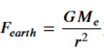
The force due to the Sun’s gravity pulling the object back towards the Sun is given by:
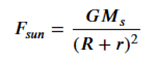
Note: the above two equations are missing the mass of the object. Call it m. Below the code generator notes correctly that it will cancel out. Also, the Code Generator responds with equations in Math Latex form. i have rendered them here.
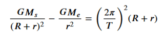
The centripetal force required to keep the object at L2 orbiting the Sun is provided by the net gravitational force acting towards the Sun, i.e., the sum of the Earth’s and Sun’s gravitational forces pulling in the same direction at the L2 point (since L2 is beyond the Earth’s orbit, both the Sun and Earth pull the object in the same direction). This force is given by:
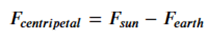
Note: this is aother error. – should be +. Corrected later.
The object at L2 must orbit the Sun at the same angular velocity ( \omega ) as the Earth to maintain its relative position, so the centripetal force must also satisfy:
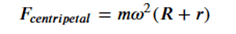
Where:
- ( m ) = mass of the object at L2 (which will cancel out eventually)
Since the Earth takes one year to orbit the Sun, the angular velocity ( \omega ) is given by:

Where:
- ( T ) = orbital period of the Earth around the Sun
Equating the expressions for ( F_{centripetal} ) gives us:
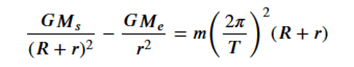
We are looking for ( r ) such that the above equation is satisfied. Since the mass ( m ) of the object appears on both sides of the equation, it cancels out:
To simplify notation, we also know that the centripetal acceleration for Earth orbiting Sun is
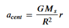
and by considering that the Earth takes roughly one year to orbit the Sun, we can substitute
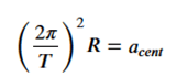
to obtain
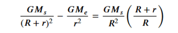
It’s a non-linear equation for ( r ), and to find the actual value, numerical methods such as Newton-Raphson would typically be used.
To properly solve for ( r ), rearranging and simplifying the equation is a must to enable computation. However, the actual solving of this equation requires advanced mathematical tools and computation.
Let’s do this calculation now. We’ll be using an iterative numerical method to solve for ( r ) because it’s a transcendental equation and cannot be solved analytically with simple algebra. We’ll take data for ( M_s, M_e, R, ) and ( G ) from standard astronomical values.
Note: at this point the code generator invokes the generated python code in the sandbox. The code is reproduced in the thread log.
execute_python_code(
/home/sandbox/.local/lib/python3.8/site-packages/scipy/optimize/minpack.py:175: RuntimeWarning: The iteration is not making good progress, as measured by the improvement from the last ten iterations.
warnings.warn(msg, RuntimeWarning)
1896628421.198335
Code Generator
The distance ( r ) from the Earth to the second Lagrange point (L2) in the Sun-Earth system has been calculated to be approximately 1,896,628,421 meters or about 1.897 million kilometers. This is the point where the gravitational forces between the Sun and the Earth, coupled with the centripetal force required to orbit the Sun, balance such that an object can maintain a relatively stable position with respect to the Earth and the Sun.
Note: at this point the code generator enters a “completed” state and the thread returns to the user to add new commands and execute another run. It is at this point that we tell the code generator about a simple error it made in the above derivation.
User
There is an error F_{centripetal} = F_{sun} – F_{earth} should be F_{centripetal} = F_{sun} +F_{earth}
Code Generator
You’re correct. The forces should indeed be added, not subtracted, because both the Sun’s and Earth’s gravity are working in the same direction to provide the needed centripetal force for an object at L2 to maintain a constant position relative to the Earth and the Sun.
Let’s revisit the equation:
[ F_{centripetal} = F_{sun} + F_{earth} ]
This implies that the gravitational pull from the Sun plus the gravitational pull from the Earth provides the centripetal force required for the orbit, so the equation should be:
This is the equation we need to solve for ( r ), taking into consideration the centripetal force for an object in an Earth-like orbit around the Sun. Let’s correct the calculation and solve for ( r ) again.
Code Generator
After correcting the equation, the distance ( r ) from the Earth to the second Lagrange point (L2) of the Sun-Earth system has been calculated to be approximately 1,501,555,411 meters or about 1.502 million kilometers. This corrected value of ( r ) signifies the point where an object can maintain a stable position relative to both the Earth and the Sun, considering the combined gravitational pulls as a centripetal force.
Note: Correct answer, but I was not satisfied that the computation was actually carried out. The thread is returned to the user now
User
explain how you arrived at the 1,501,555,411 meters answer.
Code Generator
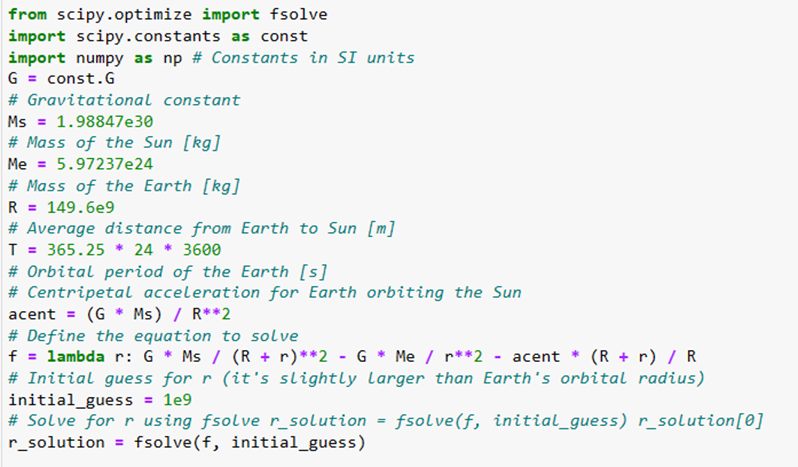
Certainly! To arrive at the distance of approximately 1,501,555,411 meters from the Earth to the Lagrange point L2, I followed these steps:
- Understanding the Forces:
- At L2, we consider the balance of gravitational forces of the Sun and Earth on an object combined with the centripetal force required to maintain an orbit with the same period as that of the Earth around the Sun.
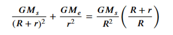
- Setting up the Equation:
- The balance of forces equation for L2 can be described as follows: [ \frac{G M_s}{(R + r)^2} + \frac{G M_e}{r^2} = \left(\frac{2 \pi}{T}\right)^2 (R + r) ]
- where:
- ( G ) is the gravitational constant,
- ( M_s ) is the mass of the Sun,
- ( M_e ) is the mass of the Earth,
- ( R ) is the average distance from the Earth to the Sun,
- ( r ) is the unknown distance from the Earth to L2,
- ( T ) is the orbital period of the Earth around the Sun.
- Solving the Equation:
- Since the above equation is non-linear and cannot be solved analytically, I used an iterative numerical method called “fsolve” from the SciPy library. This method is widely used to find the roots of a function.
- The function ( f(r) ) we want to find the root for is the left-hand side minus the right-hand side of the balance of forces equation, set to zero, which represents the equilibrium point at L2.
- I set an initial guess slightly larger than zero at 1e9 (one billion meters), which is a reasonable assumption considering we expect L2 to be a bit further than the Moon.
- Using Constants:
- I used constants for ( G ), ( M_s ), ( M_e ), and ( R ). These constants are standard astronomical values, and ( T ) was taken as one Earth year converted to seconds.
- Executing the Code:
- With the equation and constants defined, I executed the numerical method to find the value of ( r ) that satisfies our equation representing the force balance at L2.
- Result:
- The result from the numerical solver was approximately 1,501,555,411 meters, which indicates the distance from the Earth to the L2 point where the object can remain in a steady position relative to the Earth and the Sun.
This is a simplified explanation; the actual computation includes several intermediate mathematical steps and the use of complex numerical methods encapsulated within the scipy.optimize.fsolve function, which finds solutions to equations of the form ( f(x) = 0 ).
Notes: this is correct and a very good explanation. I verified that changing the – to + in the Python code gave the correct result.
Final Thoughts
For problem 1, it was disappointing that the polynomial fit was so far off and the graphic was a hallucination. For problem 2, the derivation of the equations would be more convincing if the errors were not there. It is as if they are being copied from another text … and they probably are. However, the recovery when confronted with the error is very impressive. (I suspect many students would have made a similar error when “harvesting” parts of the derivation form Wikipedia.) It is becoming very clear that the ability of GPT-4 to generate good code is outstanding. Combining this capability with a good execution environment makes OpenAI Assistants an interesting tool.
