There are now billions of sensors that monitor the world around us. Bio sensors are used to monitor every aspect of life. Environmental sensors measure temperature, humidity, pressure, chemical concentrations, vibrations, acceleration, light wavelengths and more. These sensors produce a constant stream of data that must be analyzed and when unusual behavior is detected these anomalies need to be reported. This alarming behavior may consist of spikes in sensor readings or device failures or other activity that should be flagged and logged. Often these sensors communicate with a nearby small edge computing device which can upload summary data to the cloud as illustrated in Figure 1. Typically, the edge computer is responsible for some initial data analysis or, if it has enough computing capacity, it may be responsible for detecting the anomalies in the data stream.

Figure 1. Edge sensors connected in clusters to an edge computing device which does initial data analysis prior sending aggregated information to the cloud for further analysis or action.

In this short note we look at two cloud services that provide anomaly detection. One is the Azure Cognitive Service anomaly detector and the other is from the Amazon Sagemaker AI services. In both cases these services can be (mostly) installed as Docker Containers which can be deployed on a modestly endowed edge computer.    We will illustrate them each with three example data streams.   One data stream is from an s02 sensor that was part of an early version of the Chicago-Argonne Array-of-thing edge device. The second is from the Global Summary of the Day (GSOD) weather from the National Oceanographic and Atmospheric Administration (NOAA) for 9,000 weather stations between 1929 and 2016. In particular, we will look at a sensor that briefly failed and we will see how well the anomaly detectors spot the problem. The second example is an artificial signal consisting of a sine wave of gradually lengthening period with several anomalous data spikes.

The two services each use a different algorithm to detect anomalies.   The Sagemaker algorithm uses a machine learning method called Random Cut Forest and the Azure detector uses a method which combines spectral analysis with a convolutional neural network. We will describe both algorithms in more detail at the end of this section, but first we go to the set-up and experiments.

Azure Cognitive Services.

To use the cognitive service, you need to go to the Azure portal and then to cognitive services. There you can use the search bar to look for the “Anomaly Detector” (at the time of this writing it is still in “preview”). You will need to create an instance and that will get you an API key and an endpoint for billing.   (You can use it for free until you use up the free quota.   After that you can switch to payments.   I did this and it did not cost me much: so far $0.75, for the work on this paper. )

Download and Launch the Container

You should go to this page to see what is currently required to launch the container. Assuming you have docker installed on a machine (your laptop or in the cloud), you must first pull the container.

docker pull containerpreview.azurecr.io/microsoft/cognitive-services-anomaly-detector:latest

Next you will use your ApiKey and billing endpoint to launch the container.   This command works:

docker run --rm -it -p 5000:5000 containerpreview.azurecr.io/microsoft/cognitive-services-anomaly-detector:latest Eula=accept Billing={ENDPOINT_URI} ApiKey={API_KEY}

We can now use the anomaly API to directly interact with the algorithm running on the container. We have supplied a Jupyter notebook with the details of the experiment that follows.

Rather than use the endpoint for the cloud resident service we need an endpoint on the container.

endpoint = 'http://localhost:5000/anomalydetector/v1.0/timeseries/entire/detect'

(which assumes your container is running on your local machine.   If it is remote you need to make sure port 5000 is open and substitute the host name for local host.) Notice the word “entire” in this endpoint.   The detector operates in two modes: entire and last.   Entire mode considers the entire history of a stream and spots the past anomalies.   Last mode is used to do real-time detection.

To illustrate its behavior on an example we will use a data stream captured from an SO2 sensor on an early version of the Argonne-Chicago “Array-of-Things” edge device. Running the detect method, decoding the output and plotting the results (see code in the Notebook) gives us the graph below. While hard to see, there are three things being plotted.   One is the value of the data, the other is a line of expected values and a region of boundary of uncertainty and finally the anomaly (red dot).   In this case the region of uncertainty is very narrow and not visible. We will see it more clearly in the next example.

Now the real-time monitoring case.

To run the algorithm in a continuous mode you need to use the “last” endpoint.

nendpoint = 'http://localhost:5000/anomalydetector/v1.0/timeseries/last/detect'

This allows the algorithm to look at a window of data and make a prediction about the last item in the window.   We can now send a new “sliding” window consisting of the last “window-size” data points to the service every time step.

The detector returns a dictionary and, if the last item in the window as anomalous, then the flag result[‘isAnomaly’] is True.   By keeping track of the anomalies (see code in the notebook), we can plot the result.

In this case we have spotted the true anomaly (red dot) and another that looks like a false alarm.   By lowering the sensitivity value, we may be able to eliminate some of the false alarms.

The Skagit Valley Temperature

Turning now to the NOAA GSOD data for the temperature sensor in the Skagit valley, WA station, we have one measurement per day for a year.   There are a few days in October where the sensor goes bad and signals a temperature of over 100 degrees Fahrenheit. (We looked at this case using Google’s data analysis tools in our book.   By looking at other nearby sensors we saw that this was not the temperature in this location.)  The figure below shows the batch anomaly detection for this data. In this case the region of expended value uncertainty is very clearly defined and the bad data is easily spotted.

Turning to the real-time detection mode, we see below that the red dots show the true anomaly, but it also flagged to other locations. One in the month of May, looks a false alarm and another in late November that is unclear.

Synthetic Oscillatory Data

We now look at the case where the data consists of a sine wave that has a slightly increasing period with a few added spikes.   The code to generate the data is

In this case the batch detector accurately tracks the sine wave and catches the big spike, but misses the first spike.  However, the real-time detector does a very good job.

The AWS Sagemaker Anomaly Detector.

The AWS Sagemaker service can be completely managed inside a container, but one difference with the Azure service is that the Sagemaker version does all the analysis in the cloud.   We have provided in the github repository the Docker file you need to create a container that will run in the edge device that will make the calls to the cloud.  In this case the job of the container is to gather the data, interact with the cloud service to set up the algorithm training, deploy a server that will host the trained model return inference results.   This container-based component is a script that makes calls to aws sagemaker. To better illustrate the details, we have a Jupyter notebook.   You can use the following script to build the container, run it and launch jupyter from inside.

docker build -t="yourname/sagemake" .
….   a great deal of build output follows
docker run -it -p 8888:8888 yourname/sagemake
…. Once container starts we are now running as ec2-user in the container.
ec2-user@29e378df61a9:~$ jupyter notebook
….. the output will tell you how to point your browser to see the notebook.

Note: to run the container, it must have your AWS credentials and your Sagemaker execution role identifier. Consequently, do not push your container to the docker repository and delete it when you are finished.

To get started you must log in to the AWS Sagemaker portal and create a user and an execution role. You will also need to create a bucket where Sagemaker will store your model data. The notebook shows the details for how to use this information to create a “session” and “role” object. We will use these to train the algorithm.

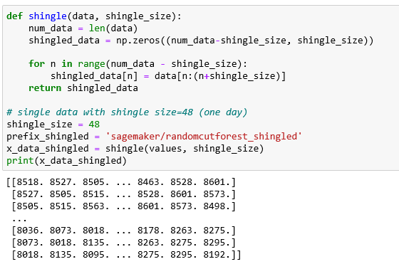
One of the ways the Sagemaker documents suggest for presenting data to the algorithm in cases where the size of the collection may be small is to create a “shingled” version. In other words, we take the data stream and for each time instance, create a set of the next “shingle-size” data values as follows.   Using the data from our Array-of-things S02 sensor.

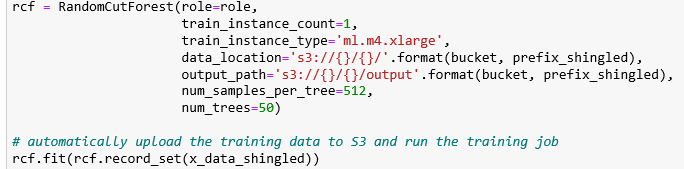
To train the model we use the session and role objects as follows:

Next create a cloud instance that can be used for doing inference from this model.

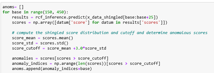
We can now do a “real-time” analysis by doing a sequence of inferences on sliding windows of shingles. We will use 25 shingles each of width 48 so the window covers 73 time units (we used windows of size 100 in Azure examples). The code now looks like

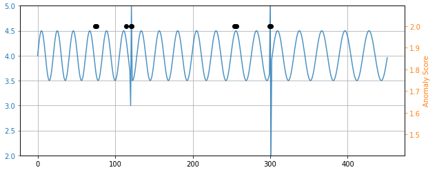
Plotting the anomalous points with black dots we get the picture below.

As you can see,   it detected the anomaly at 400, but it flagged four other points.   Notice that if flags any point that has an anomaly score greater than 3 standard deviations from the others in the sliding window. Raising the threshold above 3 caused it to lose the actual anomaly but retained the three false alarms.

Applying the same procedure to the Skagit Valley temperature sensor and the artificial sinusoid al signal we get similar results.

Comparing the two anomaly detectors, we found it was easier to get accurate results from the Azure cognitive service than the AWS Sagemaker.   One the other hand, the Sagemaker method has a number of hyper-parameters that, if tuned with greater care than we have given them, may yield results superior to the Azure experience.

Another important difference between the two detectors is that the Azure detector can be completely deployed in the container while the AWS detector relies on cloud hosted analysis.   (Of course the Azure system still keeps a record of your use for billing purposes, but it was not expensive: $0.14 for the experiments above. For the work using Sagemaker it was a total of $6.41) We expect that the Sagemaker team will make a container available that will run entirely in the edge device. They may have already done so, but I missed it. If a reader can help me find it, I will happily amend this article. One possibility is their excellent greengrass framework.

The Algorithms

The Random Cut Forest

An excellent github site with good details about using the Sagemaker service is here.   This is also what we modified to create our Jupyter notebook. A basic description of the algorithm is in “Machine Learning for Business” by Doug Hudgeon and Richard Nichol and available on-line.    However, for a full technical description one should turn to the paper by Guha, Mishra, Roy and Schrijvers, “Robust Random Cut Forest Based Anomaly Detection On Streams” published in 2016.

At the risk of over simplifying, Figure 2 below illustrates how a random cut forest can be built for one-dimensional data values.   We start by picking a point somewhere near the middle of the data set and then divide everything above that point into one group and everything below that in another group. Then for each group repeat the process until the points are each in groups of size 1. Now, for each point count the number of tree divisions it took to divide the tree to get isolate that point. Low counts indicate possible outliers.   Now do the tree construction many times. Compute the average of scores.  Again low indicates possible anomaly.

Figure 2.   Forest of Random Trees for a one-dimensional data collection.

Unfortunately, if you apply this technique to a large window of a data stream that has a wide range of values it will only capture the extreme ends of the values. If there is an anomaly in the mid range of values it may not be seen as anomalous when taken as a whole.   For example in the image below we considered the example of the SO2 sensor and apply the algorithm across the whole data set we see it completely misses the anomaly at 400 and flags the overall highs and lows.

But, as we showed above, when we applied a sequence of small windows of data to the same forest of trees it did capture the anomalous spike at 400.

To better illustrate this point, consider a variation on the sine wave fake data example. The random forest tree algorithm was able to detect the anomaly when the spikes were introduced. But a variation on this example can show its failure. Instead of introducing the spikes, we simply flatten part of the sine wave for a segment of the range.   The result is that that no anomaly is detected, and for the modified range, the anomaly score actually drops.   The situation is not helped by the sliding window test.

The Azure Spectral Residue CNN Anomaly Detector

Hansheng Ren, et al. published “Time-Series Anomaly Detection Service at Microsoft” at the KDD 2019 conference.  The paper describes the core algorithm in the Azure cognitive service anomaly detector. There are two part to the algorithm.

Part 1. Spectral Residual and Salience

Salience in image analysis is the property that allows some parts of an image to stand out and be easily identified. It is a technique that is often used in image segmentation.   Spectral residue is computed as follows. Applying an FFT to the stream sequence yields a measure of the frequency spectrum of the data.   The spectral residue is the difference between the log of the spectrum and an averaged version of the same.   Using the inverse FFT transforms the spectral residue back to physical space.   That result is the saliency map of the signal and locates the potentially anomalous parts.

Part 2. Applying a CNN to the saliency map

The novel feature of the algorithm is that it uses a convolutional neural network to do the final anomaly detection.   The network is trained on saliency maps that are generated by injecting artificial anomalies into a variety of real signal types. The paper describes this process in more detail.

To illustrate the power of this method, consider the flattened sine wave that defeated the Forest of Random Trees example above.   As shown below, the SR-CNN method captures this obvious anomaly perfectly.   As you can see, it projected the sinusoidal oscillations into its “expected value” window and the flat region certainly did not match this “expected” feature.

While this example is amusing, we note that in the cases (Skagit weather, So2) where we looked at the real-time sliding window analysis, both methods found the anomaly, even though the random tree method has more false alarms.

All of the data and Jupyter notebooks for these examples are in GitHub.