

Abstract
This tutorial gives an overview of some of the basic work that has been done over the last five years on the application of deep learning techniques to data represented as graphs. Convolutional neural networks and transformers have been instrumental in the progress on computer vision and natural language understanding. Here we look at the generalizations of these methods to solving problems where the data is represented as a graph. We illustrate this with examples including predicting research topics by using the Microsoft co-author graph or the more heterogeneous ACM author-paper-venue citation graph. This later case is of interest because it allows us to discuss how these techniques can be applied to the massive heterogeneous Knowledge networks being developed and used by the search engines and smart, interactive digital assistants. Finally, we look at how knowledge is represented by families of graphs. The example we use here is from the Tox21 dataset of chemical compounds and their interaction with important biological pathways and targets.
Introduction
Graphs have long been used to describe the relationships between discrete items of information. A basic Graph consists of a set of nodes and a set edges that connect pairs of nodes together. We can annotate the nodes and edges with the information that gives the graph meaning. For example the nodes may be people and the edges may be the relationships (married, child, parent) that exist between the people. Or the nodes may be cities and the edges may be the roads that connect the cities. Graphs like knowledge networks tend to be heterogeneous: they have more than one type of node and more than one type of edge. We are also interested in families of related graphs. For example, chemical compounds can be described by graphs where the nodes are atoms and the edges represent the chemical bonds between them.
The most famous deep learning successes involve computer vision tasks such as recognizing objects in two dimensional images or natural language tasks such as understanding linear strings of text. But these can also be described in graph terms. Images are grids of pixels. The nodes are individual pixels and edges are neighbor relations. A string of text is a one-dimensional graph with nodes that represent words and edges are the predecessor/successor temporal relationships between them. One of the most important tools in image understanding are the convolutional network layers that exploit the local neighborhood of each pixel to create new views of the data. In the case of text analysis, Transformers manipulate templates related to the local context of each word in the string. As we shall see the same concepts of locality are an essential to many of the graph deep learning algorithms that have been developed.
The Basics
Tools to manage graphs have been around for a long time. Systems like Amazon’s Neptune and Azure CosmosDB scale to very large graphs. The W3C standard Resource Description Framework (RDF) model and its standard query language, SPARQL are commonly used and well supported. Apache Tinkerpop is based on the Gremlin graph traversal language. The excellent Boost Graph Library is based on C++ generics.
These pages will rely heavily on the tools developed to manage graphs in Python. More specifically, NetworkX, originally developed by Aric Hagberg, Dan Schult and Pieter Swart, and the Deep Graph Library led by Minjie Wang and Da Zheng from AWS and Amazon AI Lab, Shanghai and a large team of collaborators (see this paper.) These two packages are complimentary and interoperate nicely. NetworkX is an excellent took for build graphs, traversing them with standard algorithms and displaying them. DGL is designed to integrate Torch deep learning methods with data stored in graph form. Most of our examples will be derived from the excellent DGL tutorials.
To begin let’s build a simple graph with 5 nodes and a list of edges stored in a file ‘edge_list_short.txt’. (the complete notebook is stored in the archive as basics-of-graphs.ipynb. We will label the nodes with their node number.

In the figure below we have the content of the edge list file on the left and the output of the nx.draw() on the right.
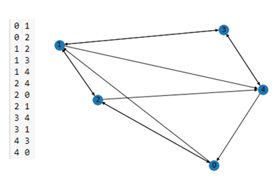
Figure 1. A simple NetworkX graph on the right derived from the short edge list on the left.
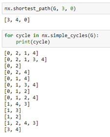
As you can see this is a directed graph. There is an edge from 4 to 0 but not one from 0 to 4. NetworkX has a very extensive library of standard algorithm. For example, shortest path computation and graph cycle detection.
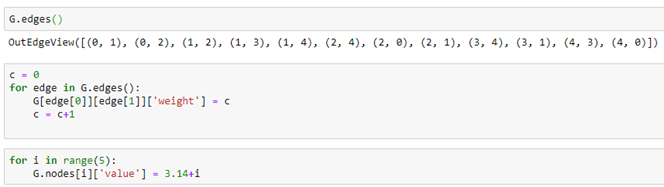
Graph nodes and edges can have properties that are identified with a property name. For example we can add an edge property called “weight” by iterating through the edges and, for each assign a value to the property. In a similar manner we can assign a “value” to each node.
DGL graphs
It is easy to go back and forth between a NetworkX graph and a DGL graph. Starting with our NetworkX graph G above we can create a DGL graph dG as follows.
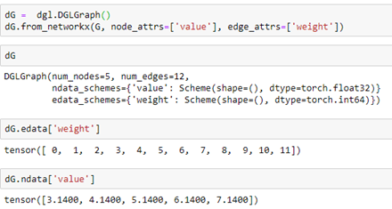
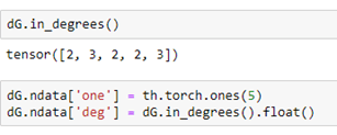
Notices that the properties “weight” and “value” are translated over to the DGL graph and Torch tensors. We can add node properties directly or using some DGL functions like out_degrees and in_degrees. Here we assign a value of 1 to a property called “one” to each node and the in degree of each node to a property called “deg”.
DGL Message Passing.
One of the most important low-level feature of DGL is the process by which messages are passed from one node to another. This is how we manage operations like convolutions and transformers on graphs.
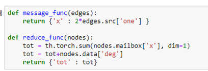
Messages are associated with edges. Each message takes a value from the source node of the edge and delivers it to the “mailbox” of the destination of the edge. Reduce functions empties the mailboxes and does a computation and modifies a property of the node. For example, the following message function just sends the 2 times the value “one” from source of each edge to the destination. After the messages are sent each node mailbox (labeled ‘x’) now has a message containing the value 2 from the nodes that have out going edge to that node. The reduce functions add up all of those 2’s (which would total twice the in-degree of that node. It then adds the in-degree again, so the value is now 3 times the in-degree of the node.
To execute these functions, we simply register the functions with our graph and invoke them with broadcast send and receive messages (with an implicit barrier between the sends and receives.)
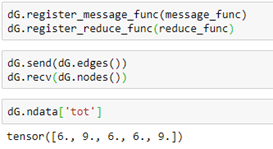
A shorthand for the send, receive pair is just dG.update_all(). The notebook for the examples above is in basics-of-graphs.ipynb in the github archive.
The MS co-author Graph
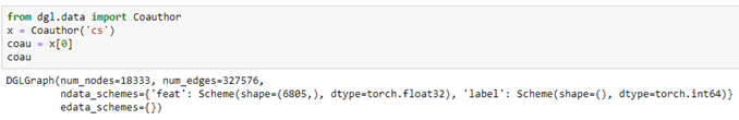
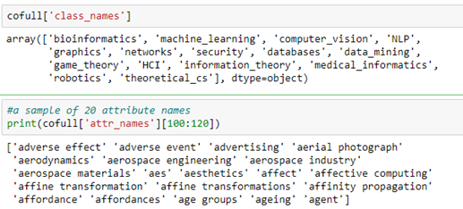
Microsoft provided a graph based on their Microsoft Academic Graph from the KDD Cup 2016 challenge 3. It is a graph of 18333 authors. Edges represent coauthors: two nodes have an edge if the authors co-authored a paper. Node features represent paper keywords for each author’s papers, and class labels indicate most active fields of study for each. There are 6805 keywords. The class labels are ‘bioinformatics’, ‘machine learning’, ‘computer vision’, ‘NLP’, ‘graphics’, ‘networks’, ‘security’, ‘databases’, ‘datamining’, ‘game theory’, ‘HCI’, ‘information theory’, ‘medical informatics’, ‘robotics’, ‘theoretical_cs’. There are two ways to get at the data. One way is from the DGL data library.
The other way is to pull the raw data collection.

There are two parts of the cofull file that are important to us. One is the array class_names and the other is the array of attributes which are the text phrases associated with each paper.
As mentioned above, the author node label is an assignment based on most likely topical research area based on publications. In the following section we will use a graph convolutional network to predict the label.
The co-author graph coau has a feature vector “feat” that describes the features for each node. This alone should be enough to predict the label.
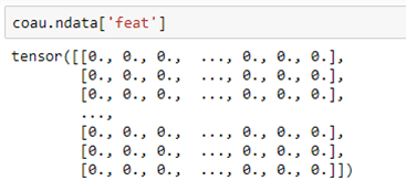
For each node this is a vector of length 6805 with a non-zero entry for each feature attribute associated with that author.
Using the cofull[‘attr_names’] list we can show what these attributes are as text. It is an interesting exercise to see what attributes are common to neighboring nodes. In the following we convert our coau graph to a NetworkX graph and look at the neighbors of node 0. Then we extract the features that several of the neighbors share with node 0. We can use the fact that the feature vector is a tensor so multiplying them together we get the intersection of the common words.
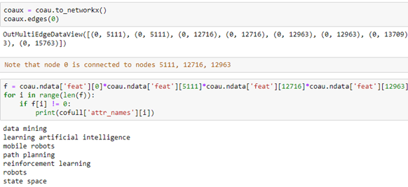
The way to read this result is that author 0 has co-authored papers with authors 5111, 12716 and 12963. Collectively they share the following phrases in their research profile.
We can create a new feature vector for each author node by extracting the list of key words on the ‘feat’ vector and constructing a Gensim tagged document.
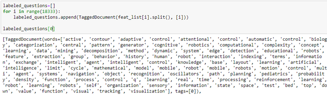
Then, using Gensim’s Doc2Vec we can create a model of vector embedding of length 100 for each of these tagged documents. These are saved in our graph in a node data feature “e-vector”.

The document model does a reasonable job of separating the nodes by class. To illustrate this we can use TSNE to project the 100 dimensional space into 2 dimensions. This is shown below for a subset of the data consisting of the nodes associated with topics ‘bioinformatics’, ‘machine learning’, ‘robotics’, ‘theoretical cs’, ‘networks’, ‘security’ and ‘databases’. The nodes associated with each topic are plotted with the same color. As you can see the topics are fairly well defined and clustered together. We will use this 100 dimension feature vector in the convolutional network we construct below.
The full details of the construction of the construction of the graph, the Doc2Vec node embedding and this visualization are in the notebook fun-with-cojauthors.ipynb
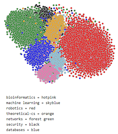
Figure 2. Subset of MS co-author graph projected with TSNE.
The Graph Convolutional Network
In computer vision applications, convolutional neural networks are based on applying filters to small local regions of each pixel. In the simplest case the template just involves the nearest neighbors to the central pixel and the template operation is a dot product with the pixel values of these neighbors.
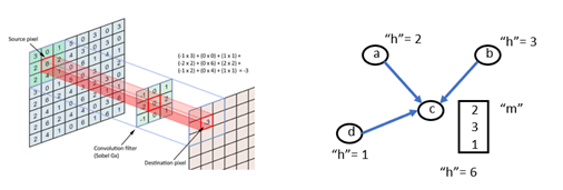
Figure 3. Convolution operations in an image and on a graph.
As shown in the figure, the graph version is the same, and we can use the DGL message system to do the computation. The standard DGL graph convolutional layer is shown below.
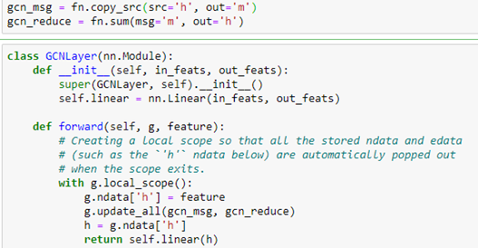
We now create a network with three GCN layers with the first layer of size 100 by 50 because 100 is the size of our new embedded feature vector we constructed with Doc2vec above. The second layer is 50 by 32 and the third is 32 by 15 because 15 is the number of classes.
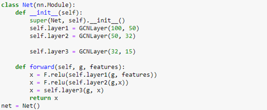
We employ a relu activation between the GNC layers. To train the network we divide the nodes into a training set and a test set by building a Boolean vector that is True when the node is in the test set and False when not. To evaluate the network on the test and train set we involve the following
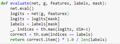
The evaluate function first applies the network to the graph with the entire feature set. This results in a tensor of size 18333 by 15. This is a vector of length 15 for each graph node. The index of the maximum value of this vector is the predicted index of the node.
To train the network we use a conventional Adam optimizer. When we extract the logits array from the network we compute the log of the soft max along the length 15 axis and compute the loss using the negative log likelihood loss function. The rest of the training is completely ordinary pytorch training.
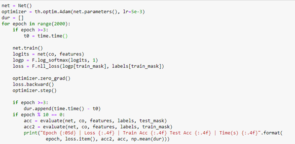
The training converged with an accuracy of 92.4%. Evaluating it on the test_mask gave a value of 86%, which is not great, but it does reflect the fact that the original graph labels are also a “subjective” valuation of the authors primary research interest.
Another way to look at the results is to plot a confusion matrix as shown below
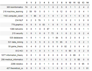
Figure 4. Confusion Matrix for prediction of topics by means of Graph Convolution Network
It is clear from looking at this that the label datamining is easily confused with databases. And the label machine-learning is often confused with computer vision and datamining. In the notebook co-author-gnc.ipynb we show how to create this matrix.
Heterogeneous Graphs
Knowledge Graphs are the basis of much of modern search engines and smart assistants. Knowledge Graphs are examples of directed heterogeneous graphs where nodes are not all of one type and edges represent relations. For example, the statement “Joan likes basketball” might connect the person node “Joan” to the sports node “basketball” and the edge from Joan to basketball would be “likes”.
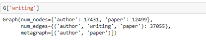
A really nice and often studied example is the ACM publication dataset. This is a collection of 12499 papers and 17431 authors and 37055 links between them. This is still small enough to load and run on your laptop. (We will discuss a much larger example later.)
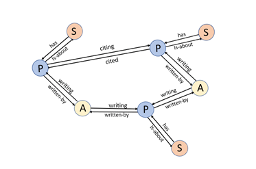
The data set consists of a set of tables and sparse matrices. The tables are ‘A’ for authors, ‘C’ for conferences, ‘P’ for papers, ‘T’ for subjects (the ACM classification), ‘V’ for proceedings and ‘F’ is for institutions. The sparse matrices are like ‘PvsA’ which means the authors of a given paper, ‘PvsP’ signifies a paper citing another, ‘PvsL’ is paper is of this topic. Downloading and creating a DGL heterograph for a subset of this data is simple.
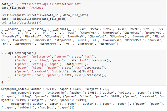
We have created a graph with three node types: authors, papers and subjects as illustrated in Figure 5 below.
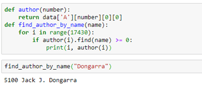
The edge types are the link keywords in the triple that is used to identify the edges. If we want to find the name of an author node we have to do a search in the data table. That is easy enough. The notebook for this example has such a trivial function:The edge types are the link keywords in the triple that is used to identify the edges. If we want to find the name of an author node we have to do a search in the data table. That is easy enough. The notebook for this example has such a trivial function:
We can use the link labels to pull out a subgraph. For example, the subgraph “authors writing paper” can be extracted by
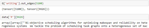
We can then ask which papers by Dongarra are included in the data set by looking for the out edges from node 5100. Having the id of the end of the out edge we can get the abstract of the paper (truncated here).
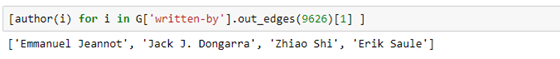
Having this information, we can use the written-by subgraph to get the names of the coauthors.
Or the subject of the paper.
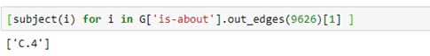
Where C.4 is the cryptic ACM code for performance of systems.
Node classification with the heterogeneous ACM graph.
The classification task will be to match conference papers with the name of the conference it appeared in. That is, given a paper that appeared in a conference we train the network to identify the conference. We have this information in the data[‘PvsC’] component of the dataset, but that was not included in our graph. There are two solutions we have considered. One is based on tranformers and is described in the excellent paper “Heterogeneous Graph Transformer” by Ziniu Hu, et. al. A notebook version of this paper applied to the ACM graph is called hetero-attention.ipynb in the Github archive. It is based on the code in their Github archive.
In the following paragraphs we will describe the version based on “Modeling Relational Data with Graph Convolutional Networks” from Schlichtkrull et. al. which is included in the DGL tutorials. The idea here is a version of the graph convolutional network. Recall that for a graph convolution each node receives a message from its neighbors and we then form a reduction sum of those messages. However for a heterogeneous graph things are a bit different. First we are interested in only one node type (paper) but each paper has several incoming edge types: author-writing-paper, paper-citing-paper, and subject-has-paper. Hence to use all the information available we must consider incoming messages from other papers as well as authors and subjects. For each edge type r we have a fully connected trainable layer W. Then for each node i and each edge type r we compute
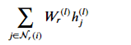
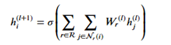
Where hj(l) is the message from the jth r-neighbor and (l) refers to the lth training iteration. Now we sum that over each edge type and apply an activation function to get
The code for this layer is below.
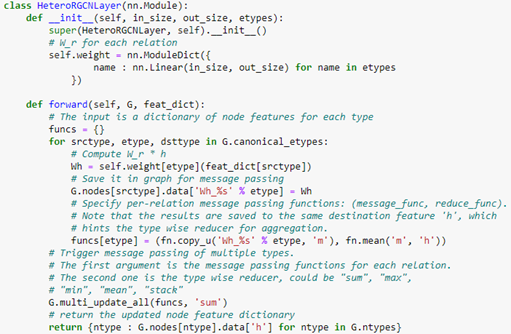
Notice that the forward method requires a feature dictionary for each node type because there are different number of nodes of each type. We construct the full network using two layers of HeteroGCN layer as follows.
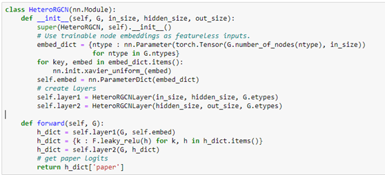
We can create our model with the following.

Where we have 4 output logits corresponding to the 4 conferences we are interested in (SOSP, SODA, SIGCOM, VLDB). We next select the rows of “PvsC” that correspond to these 4 conferences and build a train and test set from that. (The details are in our notebook GCN_hetero.ipynb .) The core of the training is quite simple and conventional.
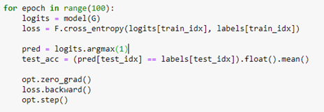
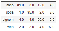
Notice that the convolutional operations are applied across the entire graph, but we only compute the loss on those node associated with our 4 selected conferences. The algorithm converges very quickly and and the accuracy on the test set is 87%. The confusion matrix shown below shows that sigcom is harder to differentiate from the others, but the size of our data set is extremely small.
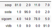
As mentioned above, we have run the same computation with the heterogeneous graph transformer algorithm. In this case the computation took much longer, but the results were slightly better as shown in the confusion matrix below.
The graphs we have presented as examples here are all small enough to run on a laptop without a GPU. However, the techniques presented here are well suited to very large graphs. For example Amazon’s AWS team we have a large scale graph based on Wikimedia with the Kensho Derived Dataset which is based on over 141 billion wikidata stements and 51 billion wikidata items. The AWS team focuses on graph embeddings at scale (see this blog) for this dataset. The have a notebook for how to access and use this data. The also use it for the Drug Repurposing Knowledge Graph (DRKG) to show which drugs can be repurposed to fight COVID-19.
Graph Classification: The Tox21 Challenge
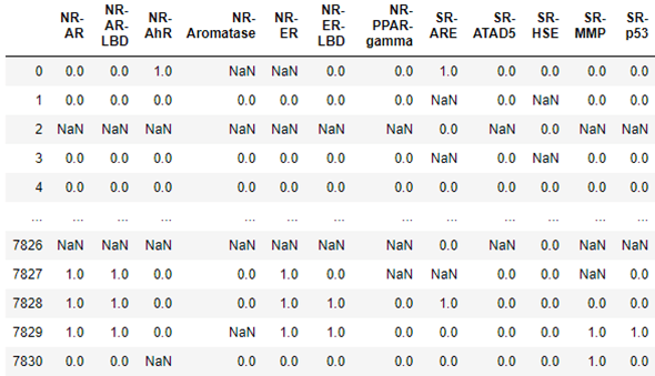
In the case of life science, Amazon has also contributed a package dgllife DGL-LifeSci. To illustrate it, we will load data associated with the Tox21 challenge from the US National Institutes of Health. This data challenge studies the potential of the chemicals and compounds being tested through the Toxicology in the 21st Century initiative to disrupt biological pathways in ways that may result in toxic effects. The dataset consists of 7831 chemical compounds that have been tested against a a compound toxicity screening classification on Nuclear Receptor Signaling (NR) and Stress Response (SR)] involving 12 different assay targets: Androgen Receptor (AR, AR-LBD), Aryl Hydrocarbon Receptor (AhR), Estrogen Receptor (ER, ER-LBD), Aromatase Inhibitors (aromatase), Peroxisome Proliferator-activated receptor gamma (ppar-gamma), Antioxidant Response Element (ARE), luciferase-tagged ATAD5 (ATAD5), Heat Shock Response (HSE), Mitochondrial Membrane Potential (MMP), and Agonists Of The P53 Signaling Pathway (P53). The table below show the result for each molecule the results of the target tests. The data is not complete, so in some cases the result are NaNs and must be excluded. As you can see below for molecule 0 there was a positive response involving receptor NR-AhR and Sr-ARE, and the Aromatase and NR_ER data was bad.
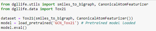
We can load the full data set, which includes the data above and a full description of each compound. In addition, we can load a pretrained graph convolutional network that attempts to predict the toxicology screen process described in the table above.
To extract the data associated with compound 0, we simply query the dataset. This returns a chemical description string (known as a smiles string), a DGL graph g, a label corresponding to the row in the table above and a mask which tells us which of the target NaN values to ignore.
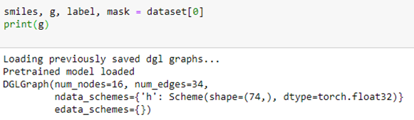
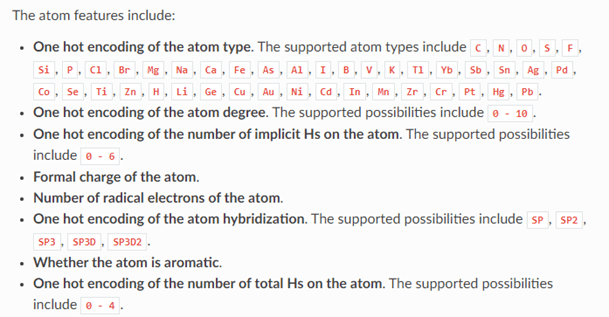
In this case the graph indicates that the chemical has 16 atoms and 34 bonds. Associated with each atom is a vector of 74 values. The meaning of these values is given below.
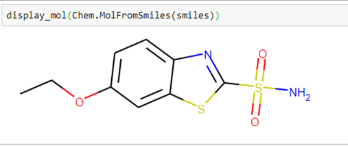
Using the smiles string and a small helper function in our notebook dgllife.ipynb called display_mol, we can see what our compound looks like.
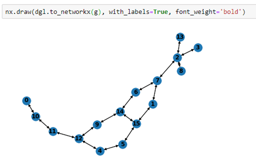
We can also draw the graph by converting it to a network graph that is graph isomorphic to the smiles graph.
As we can see from table 1 that positions 3 and 4 are no good, so using the mask we can apply the model to classify our compound.
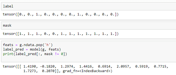
If we compare the result to the label which constitutes the correct values we see that the strongest signal is in position 5 which, after dropping two masked positions, corresponds to label position 7 in the label, which is correct. We should also get a strong signal in position 3, but we see the model gives us an even stronger signal in position 4.
Let’s look at a different compound: #7827 in the data set. This one has 23 atoms and 53 bonds.
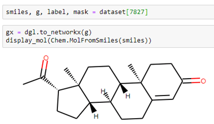
In this case, when we run the model get the following.
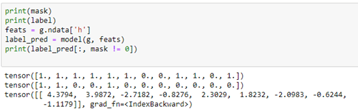
If we use the score the prediction that positive numbers indicate positive reactions (1) and negative number the opposite(0), then he predicted values are positive on the first two positions, negative on the next two and positive on the following two. This are all correct except for the last positive. The remaining three unmasked values are negative and that is correct. Out of the 9 unmasked values 8 are correct, so we can give this one a “score” of 89%. If we apply this criteria to the entire dataset we get a “score” of 83%. We did not train this model, so we don’t know what fraction of the data was used in the training, so this number does not mean much.
Conclusion
The tutorial above just scratches the surface of the work that has been done on deep learning on graphs. Among the topics that are currently under investigation include managing the updates of dynamic graphs. Of course the most interesting topic these days is the construction and use of large knowledge graphs. The big challenge there is to use a knowledge graph to do question answering. An interesting example there is Octavian’s clevr-graph which can answer questions about the knowledge graph built from the London Underground. Extracting knowledge from KGs involves understanding how to extract key phrases from English queries and how to map those phrases to KG nodes and edges. This is a non-trivial task and there is a lot of work going on.
All of the notebooks for the examples described here are in Github https://github.com/dbgannon/graphs
Some Addition References
The following are research papers and blogs that I found interesting in writing this tutorial.
- Petar Veliˇckovi´, et. al. GRAPH ATTENTION NETWORKS, arXiv:1710.10903v3
- Peter W. Battaglia, et. al. Relational inductive biases, deep learning, and graph networks, arXiv:1806.01261v3
- Michael Schlichtkrull, et. al. Modeling Relational Data with Graph Convolutional Networks, arXiv:1703.06103v4
- Alex Fouty, et. al. Protein Interface Prediction using Graph Convolutional Networks, 31st Conference on Neural Information Processing Systems (NIPS 2017), Long Beach, CA, USA.
- Xavier Bresson and Thomas Laurent, RESIDUAL GATED GRAPH CONVNETS, arXiv:1711.07553v2
- Jie Zhou, et al. Graph Neural Networks: A Review of Methods and Applications. arXiv:1812.08434v4
- William L. Hamilton, Rex Ying, Jure Leskovec, Representation Learning on Large Graphs. arXiv:1706.02216v4
- Hands-on Graph Neural Networks with PyTorch & PyTorch Geometric https://towardsdatascience.com/hands-on-graph-neural-networks-with-pytorch-pytorch-geometric-359487e221a8
- Gentle Introduction to Graph Neural Networks (Basics, DeepWalk, and GraphSage) https://towardsdatascience.com/a-gentle-introduction-to-graph-neural-network-basics-deepwalk-and-graphsage-db5d540d50b3
- https://towardsdatascience.com/how-to-do-deep-learning-on-graphs-with-graph-convolutional-networks-7d2250723780
- https://medium.com/@flawnsontong1/what-is-geometric-deep-learning-b2adb662d91d
- https://atcold.github.io/pytorch-Deep-Learning/en/week13/13-2/
