By Jack Dongarra, Daniel Reed, and Dennis Gannon
Abstract: The rapid rise of generative AI has shifted the center of gravity in advanced computing toward hyperscale AI platforms, reshaping the hardware, software, and economic landscape that scientific computing depends on. This paper argues that scientific and technical computing must “ride the wave” of AI-driven infrastructure while “building the future” through deliberate investments in new foundations. It presents seven maxims that frame the emerging reality: (1) HPC is increasingly defined by integrated numerical modeling and generative AI as peer processes; (2) energy and data movement—not peak FLOPS—are the dominant constraints, motivating “joules per trusted solution” as a primary metric; (3) benchmarks should reflect end-to-end hybrid workflows rather than isolated kernels; (4) winning systems require true end-to-end co-design, workflow first; (5) progress demands prototyping at scale with tolerance for failure; (6) curated data and trained models are durable strategic assets; and (7) new public–private collaboration models are essential in an AI-dominated market. The paper concludes with a call for a national next-generation system design “moonshot” targeting orders-of-magnitude reductions (≈1/100) in energy per validated scientific outcome via energy-aware algorithms, architecture innovation focused on memory/interconnect efficiency, and software stacks that optimize hybrid AI+simulation workflows.
1. Introduction
In 2023 [18], we argued that the center of gravity in advanced computing had already shifted away from traditional scientific and engineering high-performance computing (HPC), with the locus of influence now centered on hyperscale service providers and consumer smartphone companies. We enumerated five maxims to guide future activities in HPC:
- Semiconductor constraints dictate new approaches,
- End-to-end hardware/software co-design is essential,
- Prototyping at scale is required to test new ideas,
- The space of leading-edge HPC applications is far broader now than in the past, and
- Cloud economics have changed the supply-chain ecosystem.
Since then, given the meteoric rise of generative artificial intelligence (AI), the computing landscape has shifted more dramatically than even the most disruptive technology forecasts might have anticipated. Today, the dominant computing markets are unequivocally AI-driven; the energy and cooling demands of hyperscale systems are measured in hundreds of megawatts, making them public issues; high-precision floating point hardware is giving way to reduced precision arithmetic in support of AI models; and national strategies increasingly treat AI-capable clouds and scientific supercomputers as a fused strategic resource, with deep geopolitical implications.
Consequently, scientific and technical computing is increasingly a specialized, policy-driven niche riding atop hardware and software stacks optimized for other, much larger markets. The challenge for scientific computing is to adapt to this rapidly changing world, albeit with a more holistic perspective on the global landscape, one that looks beyond the narrow, but important design of next-generation computing systems to how an integrated ecosystem of new, nascent, and still-to-be developed computing technologies enables scientific discovery, economic opportunities, public health, and global security. We must ride the wave of AI, while simultaneously building the future.
In this paper, we outline seven new maxims that define the present and the future of advanced scientific computing. From these new maxims, we conclude with a proposal for a “moon shot” to build a new foundation for future computer systems for research, one that would benefit both scientific computing and AI..
2. Current Technical and Economic Reality
Each high-performance computing transition has been driven by a combination of market forces and semiconductor economics, requiring the scientific computing community to develop and embrace new algorithms and software to use the systems effectively. Each time, there were those who initially resisted inevitability, only to suffer the consequences of delayed adoption, whether clinging to vector supercomputers or refusing to embrace scalable message passing. Today is no different. The scientific computing community must again adapt and embrace the new realities of our AI-dominated technology world.
The first sea change is one of economic and technical influence. The scientific computing community has long been a driver of computing innovation, even in the commodity hardware space, by specifying and buying the earliest and largest instances of new technology. Today, that is no longer possible, especially under current procurement models. Today, the scale of “AI factories” dwarfs that of even the fastest machines on the list of the TOP500 supercomputers, and the gap widens each year.
Moreover, unlike the rise of the modern microprocessor, when all hardware was available for public purchase, a substantial portion of the most advanced AI hardware is designed and built by the AI hyperscalers themselves. Prominent examples include Google’s TPUs [7], Amazon’s Trainium [24], and Microsoft’s Maia hardware. The largest clusters and newest accelerator generations are often accessible only to internal AI teams within the hyperscaler or to a small set of strategic partners under commercial terms.
Although both scientific computing and generative AI benefit from high floating point operation rates, machine learning flourishes with 32, 16, 8, and even 4-bit operands. In contrast, scientific computing has long depended on high-precision, 64-bit floating point. The shift in hardware design points for hardware designed by both hyperscalers and NVIDIA, the largest supplier of AI accelerators, raises important concerns for traditional computational modeling.
In addition, the now mainstream cloud software ecosystem, including storage systems, scheduling models, and software services, differs markedly from current technical computing practices. Lest this seem heretical, remember that UNIX and open source software were once viewed as high risk by the scientific computing community, even as they became mainstream in the commercial computing world.
3. Modeling and AI As Peer Processes
Maxim One: HPC is now synonymous with integrated numerical modeling and generative AI.
The need to embrace AI is more than an economic imperative; it is also an intellectual and scientific necessity. Just as computational science became a complement to theory and experiment, later augmented by data science [25], HPC and AI are now peer processes in scientific discovery. Both are now needed to integrate deductive (computational science) and inductive (learning from data) models.
It is worth pausing to understand why there was initial resistance to AI in the computational science community. First, traditional computational simulation and modeling are deductive, based on mathematical models of phenomena based on the laws of classical or quantum physics, typically expressed as discretized differential equations. This approach reflects the classical mathematical and scientific training of most computational scientists.
In contrast, generative AI models are inductive, with models trained using large volumes of data. Just as computational models can approximate solutions to differential equations to arbitrary precision, so too can AI models learn to approximate unknown functions to arbitrary precision. Crucially, it is not a matter of choosing to invest in simulation and modeling or AI. Both are critical and complementary, each offering capabilities and efficiencies lacking in the other.
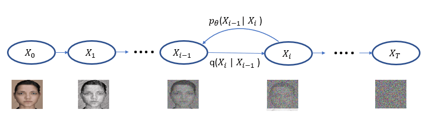
Consider weather modeling, an area long dominated by complex, numerical models. When trained on 40 years of analysis, AI can predict 10-day forecasts in seconds rather than hours, with results now competitive with the European Center for Medium Range Weather Forecasts (ECMWF) on standard metrics [11, 12, 26]. In biology, the protein folding systems, AlphaFold and RoseTTAFold, accurately predict protein 3-D structure from sequences [8,9], which many now consider to be a solved problem. AI is also a great help with inverse problems. Similarly, the AI diffusion methods used to create images can also be used to remove noise and reconstruct diagnostic-quality medical images [27]. Similar techniques can aid in searching for gravitational lensing in large scale survey data [28]. Drug and materials discovery have also been aided by AI methods that reduce search spaces prior to expensive experimentation.
Despite their great promise, AI methods are not without problems, just as numerical models face challenges regarding uncertainty quantification. Simply put, AI methods fail when applied outside the boundaries of their training data. As we noted earlier, AI methods have proven highly effective for weather prediction given historical data, but they are unable to predict the emergence of chaotic, rare events such as tornadoes. In contrast, tornadoes can now be predicted with HPC fine-grained CFD simulations, an example of the complementary utility of AI and numerical models. Nor can generative AI models readily incorporate well-known physical laws, though physics-based neural networks offer promise.
The complementary strengths and weaknesses of numerical and AI models has led to their integration as hybrid models, notably the use of AI models as numerical surrogates. First, one trains a neural network to approximate an expensive simulation, then uses the AI surrogate for rapid parameter space exploration – taking care to not push beyond its domain of applicability,, and finally uses the computationally intensive numerical simulation for verification of promising results. Similarly, for adaptive grid methods, AI can also be used to predict the region where mesh refinement may be most beneficial. These hybrid techniques incorporate the AI directly into the workflow of a large scale HPC computation.
The message is clear. AI and numerical models each have advantages and domains of applicability. Equally important, their integration creates opportunities not possible with either alone.
4. Energy and Data Movement Dominate
Maxim Two: Energy and data movement, not floating point operations, are the scarce resources.
Energy As a Design Constraint
As semiconductor scaling has slowed and architectural complexity has grown, energy consumption and heat dissipation have become limiting factors for both AI data centers and traditional supercomputers. Systems that draw hundreds of megawatts now define flagship deployments, driven by both the rising scale of deployments and the energy requirements of modern semiconductors. At these scales, every aspect of system design becomes an energy problem: how to deliver power from the grid, how to remove heat efficiently, and how to align operations with carbon reduction commitments. Liquid cooling isde rigueur with direct-to-chip, immersion, and hybrid schemes now the norm.
In this context, traditional performance metrics such as peak floating point operations per
second (FLOPS) or even time-to-solution are no longer sufficient. What matters is “joules per solution”—the total energy cost of producing a scientifically meaningful answer or training a model to an acceptable level of quality. This metric forces new trade-offs among fidelity, resolution, model size, and energy consumption. It also highlights the role of algorithmic innovation: mixed-precision methods, communication-avoiding algorithms, data compression, and smarter sampling and surrogate models can all reduce joules per solution, sometimes dramatically, without sacrificing reliability.
Critically, the time scales for computing system design and energy infrastructure decisions are increasingly mismatched. A new hyperscale data center and associated computing infrastructure can be designed and built in a few months. Upgrading power generation, transmission, or distribution infrastructure often takes much longer, especially when it involves regulatory approvals, environmental review, and large capital projects. This asymmetry means that unless the system design also includes building and operating a utility (e.g., a reactor or wind farm), the power envelope for systems is often effectively fixed years in advance, long before architectural details are finalized. As a result, future systems must be conceived as configurations that operate within pre-defined energy and cooling budgets, not as free variables to be optimized later.
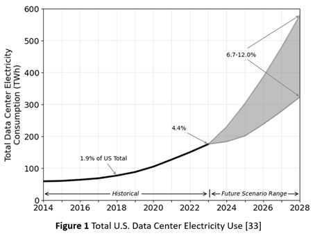
Consequently, as Figure 1 shows, the energy demand for AI factories is now outpacing the capacity of energy grids [33]. In addition to the mismatch in construction timescales, it also reflects inadequate investment, at least in the U.S., in grid modernization. Rising energy demand, from both the proliferation of data centers and their growing scale, is now a bottleneck for data center deployment. In consequence, some hyperscalers are now embracing temporary solutions, such as arrays of gas turbine generators.
Sustainability is no longer a public-relations story; it is a design constraint and an operating condition. Policy mandates, institutional climate goals, and community expectations will increasingly require large-scale computing projects to quantify and justify their energy usage in terms of joules per solution, not just peak capability. Energy efficiency must be a first-class objective across hardware, software, and workload design—not as a downstream optimization once the systems are built.
Data Movement Costs and Floating Point Arithmetic
In the past, the energy cost of arithmetic operations dominated. Today, moving data (within and between chips) consumes more energy than the arithmetic operations enabled by that data movement, yet our measures of software efficiency still center on arithmetic operation counts. Simply put, performance metrics that ignore power and communication costs encourage architectures that look impressive on paper but are increasingly impractical to operate at scale.
If facilities are to operate within tight energy envelopes while supporting both AI and high-fidelity simulation, algorithmic co-design must also extend beyond kernels and into the fundamental treatment of precision and data movement. In this view, arithmetic precision and communication are not merely implementation details; they are explicit algorithmic resources to be budgeted alongside time and memory.
This shift has already begun, with hardware designed for AI already focusing on reduced precision arithmetic to reduce energy and data movement costs. NVIDIA’s latest hardware exemplifies this trend, as illustrated in Table 1.
Operations | Peak Performance | ||
| 2022 | 2024 | 2026 | |
| NVIDIA Hopper (H200) | NVIDIA Blackwell (B200) | NVIDIA Vera Rubin | |
| FP64 FMA | 33.5 TFLOPS/s | 40 TFLOPS/s | 33 TFLOP/s |
| FP64 Tensor Core | 67 TFLOPS/s | 40 TFLOPS/s | 33 TFLOP/s |
| FP16 Tensor Core | 989 TFLOPS/s | 2250 TFLOPS/s | 4000 TFLOP/S |
| BF16 Tensor Core | 989 TFLOPS/s | 2250 TFLOPS/s | 4000 TFLOP/S |
| INT8 Tensor Core | 1979 Teraops/s | 4500 Teraops/s | 2500 Teraop/s |
| Memory bandwidth | 4.8 TB/s | 8 TB/s | 22 TB/s |
Table 1 NVIDIA Floating Point Performance
Mixed-precision methods exemplify this shift [13,14]. Rather than assuming uniform 64-bit (FP64) floating point arithmetic, future numerical solvers will partition computations across FP64, FP32, BF16, FP8, and integer-emulated formats, using high precision only where it is most needed for stability or accuracy. Iterative refinement [21], stochastic rounding [23], randomized sketching [22], and hierarchical preconditioners [20] will allow most floating point operations to be executed on low-precision units. At the same time, small high-precision components provide correction and certification. In AI workflows, similar ideas apply to training and inference, with dynamic precision schedules and quantization strategies tuned to minimize joules per unit of practical learning.
Communication-avoiding and energy-aware algorithms add a complementary dimension [15]. Classical work on minimizing messages and data movement must be reinterpreted in the context of modern communication fabrics, offload engines, and hierarchical memory systems. Runtimes will need to be aware of both energy and communication costs, scheduling tasks to minimize expensive data motion across racks or facilities and to exploit near-memory or in-network computation where possible. Hybrid AI+simulation workflows will rely on asynchronous, event-driven communication patterns that allow different parts of the system to operate at their own natural time scales without constant global synchronization.
This algorithmic work must be conducted in deliberate co-design with emerging hardware—just as hyperscalers already do for AI, where they face similar energy cost and data movement challenges [29]. Scientific computing cannot simply await new architectures and adapt afterward. Instead, targeted collaborations are needed in which hardware features (numerical precision formats, on-die networks, memory hierarchies, and DPUs) are shaped in dialogue with scientific algorithms, and in which software stacks expose those features in usable, portable ways.
5. Benchmarking and Evaluation
Maxim Three: Benchmarks are mirrors, not levers.
Performance metrics such as High-Performance Linpack (HPL), High-Performance Conjugate Gradient (HPCG), or any other next-generation benchmark reflect the systems vendors are already building; they rarely reshape the broader market trajectory on their own. Put another way, they generally reward incremental improvements rather than transformative alternatives.
New benchmarks must span both simulation and AI partitions, exercising end-to-end workflows rather than isolated kernels. For example, a climate benchmark might couple high-resolution dynamical core simulations with AI-based subgrid parametrizations and data assimilation, measuring not only time-to-solution but also energy consumed, data moved, and robustness of the resulting forecasts. A materials benchmark might link quantum-level calculations, surrogate models, and large-scale screening workflows.
Energy- and carbon-aware metrics should be central, not peripheral. Joules per trusted solution—and, where possible, estimated emissions per solution—provide a more meaningful measure of a system’s value than peak floating point performance. Benchmarks can incorporate these metrics directly, reporting performance as a Pareto frontier among time, energy, and fidelity. This will encourage architectures and algorithms that balance, rather than chasing single-number records.
Equally important is the need to benchmark the data fabric itself. Future metrics should stress test data ingestion from instruments, movement across simulation and AI partitions, access to long-term archives, and enforcement of security and access policies. They should evaluate not just raw bandwidth and latency, but also how well facilities support governed, equitable access to data and models—key concerns for national platforms that serve diverse communities.
Finally, benchmarks should reflect the hybrid nature of public-private computing infrastructure. Some workloads will span on-premise facilities and secure cloud regions; others will rely heavily on AI services coupled with local simulations. Measurement frameworks must be able to attribute performance and energy across these boundaries, enabling comparisons of different design and deployment choices.
In short, if we want design patterns for future scientific facilities that genuinely align with societal and scientific goals, we must update the mirrors we use to see ourselves. New benchmarks and metrics—rooted in AI+simulation workflows, energy and carbon efficiency, and equitable access—are as essential as new chips, racks, and cooling systems.
6. Co-Design Really Matters
Maxim Four: Winning systems are co-designed end-to-end—workflow first, parts list second.
Although the hyperscaler and AI community has aggressively embraced hardware-software co-design, in scientific computing, the story is less encouraging. There are notable examples of co-design in specific missions—fusion devices, climate modeling initiatives, and some exascale application teams have worked closely with vendors to shape features or software paths. However, most production scientific codes must still adapt to extant architectures. Porting and tuning cycles are long; exploitation of new features (tensor cores, DPUs, new memory tiers) is partial, ad hoc, and large segments of the scientific software ecosystem remain effectively frozen on older models of the machine.
Is this because the community is risk-averse, or simply because it is resource-constrained? The honest answer is both. Co-design at scale requires sustained funding, institutional continuity, and the ability to place substantial bets on uncertain outcomes. In reality, most scientific teams operate with fragmented funding and short time horizons; they cannot afford to gamble entire codes on speculative hardware features. Most tellingly, this has proven true even for the largest, mission-driven applications such as nuclear stockpile stewardship. Meanwhile, vendors are understandably reluctant to optimize for niche workloads when AI and cloud customers dominate revenue.
The net result is that co-design remains the exception rather than the rule in scientific computing. Where it has worked, it has done so in contexts that resemble AI—concentrated workloads, strong institutional commitment, and substantial aligned resources. For co-design to enable a broader spectrum of scientific codes, governance and funding structures must look more like those of AI ecosystems: fewer, more focused efforts with the scale and longevity to justify genuine hardware–software co-evolution.
7. Prototyping at Scale
Maxim Five: Research requires prototyping at scale (and risking failure), otherwise it is procurement.
In 2023 [18], we advocated for more aggressive prototyping of next-generation systems at scale. The idea was simple – if we want new architectures and programming models, ones better matched to the needs of scientific computing, we must first build and let real users test them in realistic configurations. Since then, we have seen a handful of promising large-scale prototypes and early-access systems. Nevertheless, these efforts remain scattered and, in many cases, closed or narrowly scoped, with inadequate funding and little ability to take calculated risks.
Such prototyping and development will require larger scale investments (i.e., tens of millions of dollars), either in startup companies or laboratory teams, that embrace targeted technological risks (e..g, custom chiplets) that leverage the extant hardware ecosystem. Only with scalable testbeds can new hardware, software stacks, and energy-management strategies be exercised by a wide range of scientific workloads under realistic conditions. This is neither simple nor easy, but it is essential if we are to address the limitations of hardware designed for commercial markets.
Equally importantly, advanced prototyping means being willing to accept failure while drawing lessons from the failure. Put another way, we must embrace calculated risks to explore promising new ideas. Such risk-taking was once more common in computing. One need look no further than the 1960s experiments with the IBM Stretch and the Illinois/Burroughs ILLIAC IV, followed more recently by DARPA’s targeted parallel computing program in the 1990s, which led to a host of novel parallel hardware prototypes, including the Stanford DASH and Illinois Cedar systems.
Pursued seriously, advanced prototyping may push scientific+AI HPC toward a “bespoke instrument” model. Rather than building generic machines and layering everything on top, designs might explicitly target particular classes of workflows (e.g., climate + energy systems, fusion + materials, or life sciences + health analytics) with algorithmic patterns, precision strategies, and data topologies tuned to those missions. The challenge will be to retain enough generality and openness that such bespoke instruments remain shared national resources, not single-experiment machines.
Software Stack Interoperability and Malleability
Nor can the world of prototypes be limited to software; it must also encompass interoperability between computational modeling and cloud services. In a world where traditional supercomputing and modern AI clouds are not separate worlds but interoperable layers, a climate scientist, materials chemist, or nuclear engineer would move fluidly between running large-scale simulations on government HPC systems, invoking scientific foundation models hosted in secure clouds, and using AI agents to orchestrate end-to-end workflows that span both environments.
Alternative Computing Models
Building the future means more than just riding AI hardware trends, it also means investing in alternative computing models, ones that address precisely those areas where constraints are becoming first-order: energy, data movement, and domain-specific computing.
For example, neuromorphic computing [30] can be more aptly characterized as an “energy-first” approach for event-driven, sparse inference, or control. Asynchronous, spiking networks with co‑located memory and compute are inherently suited to always‑on sensing, edge scientific instrumentation, autonomous laboratories, fast triggers, and adaptive control. The priority, not just in neuromorphic computing, but in sensing generally, really, ever since Einstein’s earliest days in physics, has been ‘act quickly, with minimal joules.’
Quantum computing [31 also represents an accelerator for a class of problems. Specifically, a quantum computer can be integrated into a hybrid processing pipeline involving chemistry/materials simulations (specific electron-structure problems), small- to medium-scale combinatorial optimization, sampling problems, and perhaps cryptology/security applications. However, the bar is relatively high, as the potential to lower the cost of communications and synchronization is becoming increasingly dominant.
8. Multidisciplinary Data Curation and Fusion
Maxim Six: Data and models are intellectual gold.
In an era when many countries can buy similar hardware and access similar cloud platforms, the differentiators are increasingly the quality of curated datasets, the sophistication of the trained models, and the legal and institutional frameworks that govern their use. High-value scientific datasets—long climate reanalyses, fusion diagnostics, high-resolution Earth observation archives, curated materials, and molecular databases—are expensive to generate and maintain.
When combined with frontier AI and hybrid AI+simulation workflows, they allow a given amount of computation to yield more insight, faster and more reliably, than would otherwise be possible. Similarly, scientific foundation models trained on such data—models for weather, climate, molecular design, materials discovery, or engineering design—become reusable assets that can be fine-tuned, coupled to simulations, and deployed across a wide range of applications.
Data stewardship must be a central element of national and institutional strategy. Investments in high-quality metadata, provenance tracking, curation, and long-term preservation are investments in future scientific leverage. Thus, the design and training of scientific foundation models must be treated as infrastructure. Just as we do not rebuild compilers and linear algebra libraries for every application, we should not treat domain foundation models as disposable experiments.
9. New Public-Private Partnerships
Maxim Seven: New collaborative models define 21st-century computing.
Frontier AI+HPC has moved from the realm of research strategy to national geopolitical policy. Executive orders and national strategies now explicitly identify AI+science platforms, secure cloud AI, and supercomputers as components of national competitiveness and security. Genesis-style [17] missions recast a historically technical conversation as a matter of national priority.
Concurrently, the shift to an AI-dominated computing market forces a rethinking of how to fund and organize scientific computing. In a world where hyperscalers and AI platform companies set the pace of hardware innovation, traditional models—incremental upgrades to on-premise systems funded through periodic capital campaigns—are no longer sufficient to sustain leadership in HPC for science. Instead, future government funding models must recognize that advanced computing is now a mixed public–private ecosystem, in which strategic consortia, pre-competitive platforms, and mission-driven initiatives play central roles.
In turn, this means articulating explicit AI+HPC requirements linked to national and global challenge problems – climate resilience, health, energy transition, national security, and economic competitiveness. Funding calls that tie hardware, software, data, and workforce development together—anchored in concrete mission outcomes—are more likely to produce durable ecosystems than one-off hardware acquisitions.
Genesis-style initiatives are one example of this logic: they frame AI+science platforms as critical infrastructure for national goals rather than as isolated technology experiments. The core lesson is that publicly funded scientific computing cannot succeed by passively purchasing available computing hardware. It needs proactive, coalition-based funding models that treat AI+HPC as a long-term strategic national asset, integrating hardware, software, data, and people under coherent missions.
10. Implications for the Future
The old model of HPC as a dominant, self-directed driver of advanced hardware and software has ended. Indeed, it arguably ended decades ago, with the emergence of clusters based on commodity microprocessors. Absent strategic investment in new architectures, what remains is a role dependent on AI-centric, hyperscaler investments for technology advances.
In such a world, Genesis is a pragmatic bridge into the AI-factory era, but it should not become the ceiling of our ambition. “AI factories” cannot continue growing without bounds; there are practical energy and carbon constraints. Equally importantly, the future trajectory of semiconductor innovation and cost curves is also uncertain.
If the dominant commercial trajectory is toward ever larger, ever more energy-intensive clusters (e.g., xAI-style “Colossus” builds, Oracle’s OCCI-class deployments, and other zettascale-aspirational AI campuses), then science needs a countervailing national program whose primary objective is not peak capability, but orders-of-magnitude reduction in joules per trusted solution.
We believe the scientific computing community must play a distinctive role in reshaping this ecosystem. This includes serving as a co-designer of AI infrastructure, drawing on decades of experience in numerical methods, performance engineering, and uncertainty quantification to collaborate on the design of AI-centric systems that support both scientific computing and AI-mediated discovery. Doing so will require embracing new models of collaborative public-private partnership, identifying leverage points where early research can shape technology futures.
11. A Call To Action: A National Next-Generation System Design Moonshot
Consider the following Gedanken challenge: deliver the same validated scientific results as today’s frontier AI datacenters, but at roughly 1/100th the energy per solution? Such a target requires a fundamentally different design point that includes: energy-proportional computing [32], extreme data-movement frugality, and algorithm-architecture co-design that treats numerical precision, communication, and verification as first-class resources, not afterthoughts.
Why has this not been the default design point, and a sociotechnical imperative, given the clear and ever more looming challenges of today’s approach? Simply put, because it is far more challenging than incrementalism and procurement. A true moonshot requires accepting risk (and failure), building prototypes early, and resisting the temptation to equate “national leadership” with the largest single installation. It also challenges existing incentives: vendors optimize for hyperscale utilization; government procurement cycles favor incremental upgrades; and “largest machine” headlines still crowd out efficiency metrics.
The scientific case for such a moonshot is compelling. AI factories and HPC systems face similar technical challenges, including inadequate memory bandwidth, high and rising energy requirements, and semiconductor scaling issues. Moreover, many of the highest-value workflows (i.e., climate and weather ensembles, materials screening, fusion design loops, health analytics, inverse problems, and hybrid AI+simulation pipelines) scale best when one can run many jobs in parallel with predictable energy cost. A fleet of smaller, efficient systems can deliver more scientific throughput per dollar and per megawatt than a single monolithic machine, while improving resilience, availability, and breadth of access.
Note that we are not suggesting that we abandon the desire for higher performance, merely that our current approach to increasing performance has reached the point of diminishing returns. We must first rebuild the foundations of computing, then leverage these foundations to build both leading edge systems and a set of grid-deployable “science engines” – modular systems small enough to locate at multiple research institutions and regional power nodes, and numerous enough to support diverse communities.
In many ways, computing became most transformative when it became small enough and economical enough for personal use; the national analogue is to make advanced capability compact, repeatable, and ubiquitous enough that science can own the workflows end-to-end. The same is true for AI engines; broad access is needed for scientific discovery.
Concretely, such a moonshot would couple (i) aggressive energy-aware algorithms (mixed precision with certification, communication-avoiding methods, learned surrogates with validation), (ii) architecture innovation focused on memory and interconnect efficiency rather than raw FLOPS, and (iii) software stacks that measure and optimize joules per trusted outcome across hybrid AI+simulation workflows. The outcome of such a project would not replace Genesis; it would complement it, making sure that public science is not forever constrained to renting computing and storage resources designed for someone else’s business model.
References
[1] G. E. Moore, “Cramming More Components Onto Integrated Circuits,” Electronics, vol. 38, no. 8, pp. 114–117, Apr. 1965. DOI: https://doi.org/10.1109/JSSC.1965.1051903
[2] J. L. Hennessy and D. A. Patterson, Computer Architecture: A Quantitative Approach, 6th ed. Morgan Kaufmann, 2019.
[3] R. H. Dennard, F. H. Gaensslen, H.-N. Yu, V. L. Rideout, E. Bassous, and A. R. LeBlanc, “Design of Ion-Implanted MOSFET’s with Very Small Physical Dimensions,” IEEE Journal of Solid-State Circuits, vol. 9, no. 5, pp. 256–268, 1974. DOI: https://doi.org/10.1109/JSSC.1974.1050511
[4] J. Dongarra et al., “The International Exascale Software Project Roadmap,” International Journal of High Performance Computing Applications, vol. 25, no. 1, pp. 3–60, 2011. DOI: https://doi.org/10.1177/1094342010391989
[5] OpenAI, “AI and Compute,” OpenAI Blog, 2018.
[6] T. B. Brown et al., “Language Models are Few-Shot Learners,” Advances in Neural Information Processing Systems, vol. 33, 2020.
[7] N. P. Jouppi et al., “In-datacenter Performance Analysis of a Tensor Processing Unit,” in Proc. 44th ACM/IEEE Annual International Symposium on Computer Architecture (ISCA), 2017. DOI: https://doi.org/10.1145/3079856.3080246
[8] J. Jumper et al., “Highly Accurate Protein Structure Prediction with AlphaFold,” Nature, vol. 596, no. 7873, pp. 583–589, 2021. DOI: https://doi.org/10.1038/s41586-021-03819-2
[9] M. Baek et al., “Accurate Prediction of Protein Structures and Interactions Using a Three-Track Neural Network,” Science, vol. 373, no. 6557, pp. 871–876, 2021. DOI: https://doi.org/10.1126/science.abj8754
[10] G. Carleo et al., “Machine Learning and the Physical Sciences,” Reviews of Modern Physics, vol. 91, no. 4, p. 045002, 2019. DOI: https://doi.org/10.1103/RevModPhys.91.045002
[11] S. Rasp, M. S. Pritchard, and P. Gentine, “WeatherBench: A Benchmark Dataset for Data-Driven Weather Forecasting,” Journal of Advances in Modeling Earth Systems, vol. 12, no. 11, 2020. DOI: https://doi.org/10.1029/2020MS002203
[12] R. Nguyen et al., “Learning Skillful Medium-Range Global Weather Forecasting,” Science, vol. 382, pp. 1416–1422, 2023. DOI: https://doi.org/10.1126/science.adi2336
[13] N. J. Higham, “Accuracy and Stability of Numerical Algorithms,” 2nd ed. SIAM, 2002. DOI: https://doi.org/10.1137/1.9780898718027
[14] A. Haidar, S. Tomov, J. Dongarra, and N. Higham, “Harnessing GPU Tensor Cores for Fast FP16 Arithmetic to Speed Up Mixed-Precision Iterative Refinement Solvers,” in Proc. SC18, 2018. DOI: https://doi.org/10.1109/SC.2018.00034
[15] J. Demmel, L. Grigori, M. Hoemmen, and J. Langou, “Communication-Avoiding Algorithms,” Acta Numerica, vol. 23, pp. 1–111, 2014. DOI: https://doi.org/10.1017/S0962492914000038
[16] U.S. Congress, “CHIPS and Science Act of 2022,” Public Law 117-167, Aug. 9, 2022.
[17] Executive Office of the U.S. President, “Executive Order on the American Science and Security Platform and the Genesis Mission,” Washington, DC, 2025, https://www.whitehouse.gov/presidential-actions/2025/11/launching-the-genesis-mission/
[18] Reed. D., Gannon, D., Dongarra, J., “HPC Forecast: Cloudy and Uncertain,” Communications of the ACM, Vol. 66, No. 2, pp. 82-90, https://doi.org/10.1145/3552309, January 2023.
[19] Price, I., Sanchez-Gonzalez, A., Alet, F. et al. Probabilistic Weather Forecasting with Machine Learning. Nature 637, 84–90 (2025). https://doi.org/10.1038/s41586-024-08252-9
[20] Halko, N.; Martinsson, P.-G.; Tropp, J. A. “Finding Structure with Randomness: Probabilistic Algorithms for Constructing Approximate Matrix Decompositions.” SIAM Review, 2011. DOI: 10.1137/090771806.
[21] Abdelfattah, Anzt, Boman, Carson, Cojean, Dongarra, et al. A Survey of Numerical Linear Algebra Methods Utilizing Mixed-Precision Arithmetic, Int’l J. High Performance Computing Applications (2021). DOI: 10.1177/10943420211003313.
[22] Riley Murray, James Demmel, Michael W. Mahoney, et al., “Randomized Numerical Linear Algebra: A Perspective on the Field With an Eye to Software” (arXiv:2302.11474v2, Apr 12, 2023).
[23] Croci, Fasi, Higham, Mary, Mikaitis, “Stochastic Rounding: Implementation, Error Analysis and Applications,” Royal Society Open Science, 2022. DOI: 10.1098/rsos.211631.
[24] Xinwei Fu, Zhen Zhang, Haozheng Fan, Guangtai Huang, Mohammad El-Shabani, Randy Huang, Rahul Solanki, Fei Wu, Ron Diamant, and Yida Wang, Distributed Training of Large Language Models on AWS Trainium, SoCC ’24: Proceedings of the 2024 ACM Symposium on Cloud Computing, pp. 961-976, https://doi.org/10.1145/3698038.369853
[25] Tony Hey, Stewart Tansley, and Kristin Tolle, eds., The Fourth Paradigm: Data-Intensive Scientific Discovery (Redmond, WA: Microsoft Research, 2009).
[26] Remi Lam, Alvaro Sanchez-Gonzalez, Matthew Willson, Peter Wirnsberger, Meire Fortunato, Ferran Alet, Suman Ravuri, Timo Ewalds, Zach Eaton-Rosen. Weihua Hu, Alexander Merose, Stephan Hoyer https://orcid.org/0000-0002-5207-0380, George Holland, Oriol Vinyals, Jacklynn Stott, Alexander Pritzel, Shakir Mohamed, and Peter Battaglia. Learning Skillful Medium-Range Global Weather Forecasting,” Science, 382,1416-1421(2023).DOI:10.1126/science.adi2336
[27] Mohammed Alsubaie, Wenxi Liu, Linxia Gu, Ovidiu C. Andronesi, Sirani M. Perera, and Xianqi Li, “Conditional Denoising Diffusion Model-Based Robust MR Image Reconstruction from Highly Undersampled Data,” March 2025, https://arxiv.org/html/2510.06335v1
[28] Supranta S. Boruah and Michael Jacob, “Diffusion-based Mass Map Reconstruction From Weak Lensing Data,” February 2025, https://arxiv.org/html/2502.04158
[29] Xiaoyu Ma and David Patterson, “Challenges and Research Directions for Large Language Model Inference Hardware,” https://arxiv.org/abs/2601.05047, 2026
[30] Dennis V Christensen, Regina Dittmann, Bernabe Linares-Barranco, Abu Sebastian, Manuel Le Gallo, Andrea Redaelli, Stefan Slesazeck, Thomas Mikolajick, Sabina Spiga, Stephan Menzel, “2022 Roadmap on Neuromorphic Computing and Engineering, ”022 Neuromorphic Computing and Engineering, 2 02250, DOI 10.1088/2634-4386/ac4a83, 2022
[31] National Academies of Sciences, Engineering, and Medicine. Quantum Computing: Progress and Prospects. National Academies Press, 2019 (DOI: 10.17226/25196).
[32] Luiz A. Barroso and U. Hölzle, “The Case for Energy-Proportional Computing,” IEEE Computer, 40 (12): 33–37. doi:10.1109/mc.2007.443. S2CID 6161162, 2007
[33] Arman Shehabi, Sarah Josephine Smith, Alex Hubbard, Alexander Newkirk, Nuoa Lei, Md AbuBakar Siddik, Billie Holecek, Jonathan G Koomey, Eric R Masanet, and Dale A Sartor, “2024 United States Data Center Energy Usage Report,” Lawrence Berkeley National Laboratory, DOI 10.71468/P1WC7Q, 2024
Jack Dongarra is Professor Emeritus at the University of Tennessee, EECS Department, Knoxville, Tennessee, USA and Univeristy of Manchester, UK.
Daniel Reed is a Presidential Professor at the University of Utah, Computer Science and Electrical & Computer Engineering, Salt Lake City, Utah, USA.
Dennis Gannon is Professor Emeritus at the Indiana University, Luddy School of Informatics, Computing and Engineering, Bloomington, Indiana, USA.