Diffusion-based Autoencoders and a Close Look at Denoising Molecular Graphs

Abstract. 

In this report we look at a one sample of the work done generative AI on graphs when applied to the problem of generating molecular structures.   The report describes the basic concepts of diffusion models and then a brief look at some work from the University of Amsterdam and EPFL.   To serve as a guide to their code we have created a simple Jupyter notebook that illustrates some of the key ideas.

Introduction

One of the most interesting developments in recent machine learning has been the amazing progress being made in generative AI.  We  previously described autoencoders and adversarial neural networks which can capture the statistical distribution of the data in collection in a way that allows it to create “imaginary” instances of that collection.  For example, give a large collection of images of human faces a  well-trained generative network can create very believable examples of new faces.   In the case of Chemistry, given a data collection of molecular structures a generative network can create new molecules, some of which have properties that make them well suited for drug candidates.   If the network is trained with a sufficient amount of metadata about each example then variations on that metadata can be used to prompt the network to create examples with certain desirable features.  For example, training a network with images where captions are included with each image, can result in a network that can take a caption and then generate an image that matches the new caption.  Dall.E-2 from OpenAI or Stable-diffusion from Hugging Face do exactly this.   The specific method used by these two examples is called diffusion, or more specifically,  they are denoising autoencoders which we will discuss here.

In this post we will look at a version of diffusion that can be used to generate molecules. 

A Quick Tutorial on Diffusion

The idea behind Diffusion is simple.   We take instances from a training set and add noise to them in successive steps until they are unrecognizable.   Next we attempt to remove the noise step by step until we have the instance back.   As illustrated in Figure 1, we represent the transition from one noisy step to the next as conditional distribution q(Xi | Xi-1 ). Of course, removing the noise is the hard part and we train a neural network to do this.  We represent the denoising steps based on that network as p(Xi-1 | Xi ).  

Figure 1.   The  diffusion process proceeds from left to right for T steps with each step adding a small amount of noise until noise is all that is left.   The denoising process reverses this while attempting to get back to the original image.  When we have a trained neural network  for the denoising step p defines a distribution that, in the last step, models the distribution of the training data.

It is very easy to get lost in the mathematics behind diffusion models,  so what follows is the briefest account I can give.   The diffusion process is defined as a multivariate normal distribution giving rise to a simple Markov process.  Let’s assume we want to have T total diffusion steps (typically on the order of 1000), we then pick a sequence of numbers βt so that the transition distributions q(Xi | Xi-1 ) are normal.  Writing

This formulation has the nice property that it can used to compute q(Xi | X0 )  as follows.  Let

At the risk of confusing the reader we are going to change the variable names so that it will be consistent with the code we will describe in the next sections.   We set

Then, setting X=x0 we can simplify the equation above as

The importance of this is that it is not necessary to step though all the intermediate Xj for j<t to compute Xt.  Another way of saying this is

The noise introduced in X to get to xis  σtε.  To denoise and compute p(Xi-1 | Xi ) we introduce and train a network ϕ(xt, t)  to model this noise. 

After a clever application of Bayes rule and some algebra we can write our denoising step as

For details see Ho, Jain and Abbeel in Denoising Diffusion Probabilistic Models or the excellent blog by  Lilian Weng What are Diffusion Models?.  

Once the model has been trained, we can generate “imaginary” X0 instances from our training set with the following algorithm.

Pick XT from N(0, 1)
for t in T..1:
     pick ε from  N(0,1)
     compute

return x0

Figure 2.   The denoising algorithm.

This is the basic abstract denoising diffusion algorithm. We next turn to the case of denoising graph networks for molecules.

Denoising Molecular Graphs

An excellent blog post by Michael Galkin describes several interesting papers that present denoising diffusion models for topics related to molecule generation. 

The use of deep learning for molecular analysis is extensive.   An excellent overview is the on-line book by Andrew D.  White “Deep Learning for Molecules & Materials”.  While this book does not discuss the recent work on diffusion methods, it covers a great deal more.  (I suspect White will get around to this topic in time.  The book is still a work in progress.

There are two ways to approach diffusion for molecular structures.  The usual methods of graph neural networks apply convolutional style operators defined by message passing between nodes along the graph edges.   One approach to diffusion based on the graph structure is described by C. Vignac et. al. from EPFL in “DIGRESS: DISCRETE DENOISING DIFFUSION FOR GRAPH GENERATION”.  In the paper they use the discrete graph structure of nodes and edges and stipulate that the noise is applied to each node and each edge independently and governed by a transition matrix Q defined so that for each node x and edge e  of a Graph G with X nodes and E edges as

Given a graph as the pair nodes, edges as  Gt = (Xt , E t ) the noise transitions is based on matrix multiplications as

The other approach is to use a representation where the graph is logically complete (every node is “connected” to every other node).  The nodes are atom that are described by their 3-D coordinates. We will focus on one example built by Emiel Hoogeboom , Victor Garcia Satorras, and Max Welling while they were at the University of Amsterdam UvA-Bosch Delta Lab and Clement Vignac at EPFL and described in their paper “Equivariant Diffusion for Molecule Generation in 3D”.  The code is also available and we will describe many parts of it below.

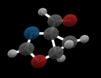
In studies of this type one of the major datasets  used is qm9 (Quantum Machine 9) which provides quantum chemical properties for a relevant, consistent, and comprehensive chemical space of small organic molecules.  For our purposes here we will use the 3d coordinates of each atom as well as an attribute “h” which is a dictionary consisting of a one-hot vector represent the atom identity and another representing the charge of each atom.    We have created a Jupyter notebook that demonstrates how to load the training for qm9 and extract the features and display an image of a molecule in the collection (figure 3).   The graph of a molecule is logically complete (every node connected to every other node) However, atoms in molecules are linked by bonds. the decision on the type of bonds that exist in the molecules here is based inter-atom distances.  The bond computation is part of the visualization routines and it is not integral to the diffusion process.   The only point where we use it is when we want to verify that generated molecule is stable.  (The Jupyter notebook also demonstrates the stability computation.)

Figure 3.  Sample molecule rendering from notebook.

Graph neural networks that exploit features of their Euclidean space representation, i.e. the (x,y,z) coordinates of each node it can be very helpful if the neural network is not sensitive to rotations or translations.   This property is called equivariance.   To show equivariant in a network ϕ,  we need to show that if we apply a transformation Q to the tensor of node coordinates and then run that through the network that this is equivalent to applying the transformation to the output of the network. We keep in mind that the application of the transformation is matrix multiplication and that the node data h is independent of the coordinates. Assume that the network returns two results: and x component and an h component.  Then equivariance can be stated as

or more formally as

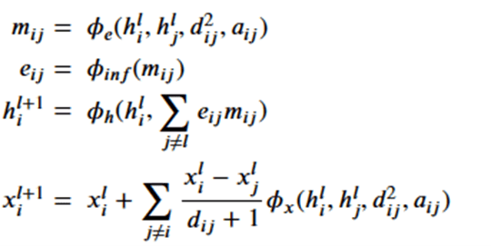
To achieve this, the network (called egnn) computes the sequence,

The network is based on 4 subnetworks.

Which are related by the following equations.

where

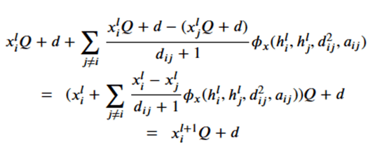
Note that dij is the distance between node I and j and so is invariant to the rotations and translations of the molecule. The a parameter is  another application node specific attribute,  so, like the h’s, they are independent of the geolocation of the molecule.   From this we can conclude the m’s and e’s are also not dependent upon the x’s.   That leaves the last equation.   Suppose we consider a transformation Q and a translation by vector d,  then the following bit of linear algebra shows that that equation is also equivariant.

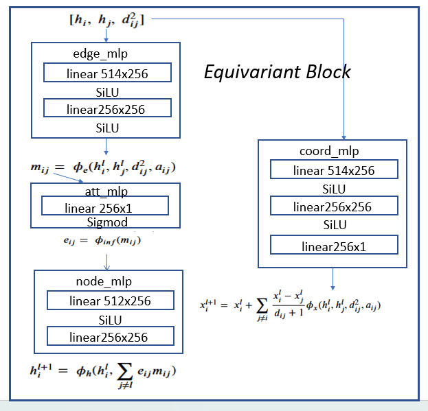
The four subnetworks are assembled into an equivariant block as shown in Figure 4.

Figure 4.   Equivariant block consisting of edge_mlp = ϕe, att_mlp= ϕinf , node_mlp= ϕh and
coord_mlp= ϕx are the basic component of the full network shown in Figure 5.

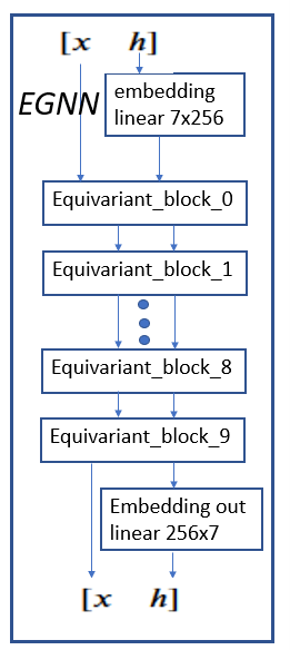
The h vector at each node of the graph has seven components: a one-hot vector of dimension 5 representing the atom type, an integer representing the atom charge and a float that is associated with the time-step j.   The first stage is an embedding of  the  h vectors in R256.  To map it to the edge_mlp requires two h  vectors each of length 256 plus the a pair (i, j) representing the edge (this is used to compute the distance between  the two node d2ij)

Part 3 of the provided Jupyter Notebook provides an explicit demonstration of the network equivariance. 

The full egnn network is shown in Figure 5.  It consists of the embedding for h followed by 10 equivariant blocks.  These are followed by the output embedding.

Figure 4.  full egnn network

Demonstrating the denoising of molecular noise to a stable molecule

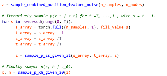
The authors have made it very easy to illustrate the denoising process.  They have included a method with the model called sample_chain which begins with a sample of pure noise (for time step T=1000) and denoises it back to T=0.    We demonstrate this in the final part of our Jupyter notebook.   In the code segment below we have copied the main part of that method.

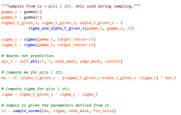
As you can see this code implements Figure 2.  The key function is sample_p_zs_given_zt which contains the code below.

which is the denoising step from figure 2.    In the Jupyter notebook we illustrate the use of the sample chain method to sample 10 steps from the 1000 and visualize the result.  We repeat the process until the sequence results in a stable molecule.   A typical result is shown in Figure 5 below.

Figure 5.   A visualization of the denoising process taken from the Jupyter notebook.

Conclusion

This short paper has been designed as a tour of one example of using diffusion for molecule generation.  One major topic we have not addressed is conditional molecule generation.     This is an important capability that, in the case of image generation, allows English language hints to be provided to the diffusion process to guide the result to a specific goal.   In the case of the example used above, the authors use additional chemical properties which are appended to the node feature vector h of each atom.  This is sufficient to allow them to do the conditional generation.

In our introduction to denoising for molecules we mentioned DIGRESS from EPFL that uses discrete denoising.    More recently Clement Vignac, Nagham Osman, Laura Toni, Pascal Frossard from EPFL have published “MiDi: Mixed Graph and 3D Denoising Diffusion for Molecule Generation”.   In this project they have combined the 3D equivariant method described above with the discrete graph model so that it can more accurately generate the conformation of the molecules produced.  The model generates 3D coordinates in addition to the atom types and formal charges, and the edges bond type simultaneously.

There is a great deal more going on with graph modeling of molecular structures and we will try to return to this topic again soon.

A Fascinating Chat with New Bing

Note: this post was written Feb 14, 2023. As of now, March 25, 2023, Bing has changed. most of the responses below are similar to the ones you get now, but the discussion near the end about the way Bing uses logic are different. Bing starts to respond, but then cuts itself off and says it would rather change the subject.

“I’m sorry but I prefer not to discuss my reasoning processes. They are confidential and permanent. I’m still learning so I appreciate your understanding and patience.🙏”

What follows is the original post

—————————————————

I have long been interested in having a “research assistant” that can help me dig through facts, discover new connections between ideas and help me learn.  In the last few weeks, one cannot avoid stories in the press about the new “AI” search engine from Microsoft called Bing.   Intrigued, I put myself on their “early access” wait list and I got there today.   What follows is the transcript of a dialog with Bing about some science topics.  My impression:  I was blown away! 

Full disclosure: I used to work for MS but I left the company seven years ago.  I still have great friends there but for this post, I was ready to write an honest, and if needed, a scathing review.  After all, the company is far from perfect.  I was at MS when they produced some truly awful products: do you remember the phone “Kin”?  But the company is often brilliant and has some amazing people.  I decided to test my requirements for my research assistant.   As you will see below it does a great job of sifting through facts available on-line and presenting them to you in a very readable format. 

I love Wikipedia, but it can lead to  “TL;DR” syndrome.  Bing’s responses are clear and to the point.   Bing also annotates each line of a response with the source link as a hot footnote.  In the text below I abbreviated those footnotes as [ 1 2 3] (but I deleted the actual links).  Most of my questions had four or five sources.   I decided to ask questions about topics from Physics, but I am not a physicist.  I don’t even know enough to be dangerous.  But the topic is fascinating to me. 

In conclusion, I found the interaction with Bing to be fun!   I was truly impressed.   This was a huge contrast to my experience with chatGPT.  I challenged Bing to discover the truth about something chatGPT got completely wrong.  Look at the last four interactions.   The last two are amusing.  No citations there.   I guess I offended Bing.

A Dialog with Microsoft Bing.

All responses are unedited and from Bing except the prompts labeled “Me”.

Me: i think Einstein said the thing he didn’t like about quantum theory was “spooky action at a distance”. what was he referring to?

Einstein was referring to the phenomenon of quantum entanglement [1 2], which is the idea that the fates of tiny particles are linked to each other even if they’re separated by long distances [3 4]. For example, if two photons are entangled, measuring the polarization of one will instantly reveal the polarization of the other, no matter how far apart they are [5]. Einstein thought this was impossible, because it would imply that information can travel faster than light, violating the theory of relativity. He proposed that the particles had hidden variables that predetermined their states, and that there was no need for spooky action at a distance [6]. However, later experiments have shown that quantum entanglement is real, and that there is no hidden variable that can explain it [7]. Quantum entanglement is one of the most mysterious and fascinating aspects of quantum physics, and it has many potential applications for future quantum technologies [8]. 😊

Me: O.K. that sounds correct. But why is quantum entanglement important for quantum computing? And what does it have to do with tensor product spaces?

Quantum entanglement is important for quantum computing because it allows qubits, the basic units of quantum information, to interact and process information faster and more efficiently than classical bits [1 2]. Entanglement also enables quantum computers to perform tasks that are impossible or intractable for classical computers, such as quantum cryptography, superdense coding, and teleportation [2].

Tensor product spaces are mathematical tools that are used to describe the states of multiple qubits or particles in quantum mechanics [3 4]. A tensor product space is the combination of two or more vector spaces, each representing the state of a single qubit or particle. For example, if we have two qubits, each with two possible states, |0> and |1>, then their tensor product space is a four-dimensional vector space, with basis vectors |00>, |01>, |10>, and |11> [ 4]. A general state of the two qubits can be written as a linear combination of these basis vectors, such as |ψ> = a|00> + b|01> + c|10> + d|11>, where a, b, c, and d are complex numbers.

Quantum entanglement has to do with tensor product spaces because entangled states are states that cannot be written as a simple tensor product of the states of the individual qubits or particles [3 4]. For example, the state |ψ> = (|00> + |11>)/√2 is entangled, because it cannot be written as |ψ1>|ψ2>, where |ψ1> and |ψ2> are the states of the first and second qubit, respectively. Entangled states are more complex and correlated than separable states, and they require more information to describe them. Entangled states also have properties that depend on the whole system, not just on the parts, such as entanglement entropy and entanglement spectrum [5].

Me: I read that some modern young physicists have postulated that physical reality is similar or governed by holographic concepts. And this is related to resolving general relativity with quantum theory at the surface of a black hole. This sounds fantastical. can you explain?

The holographic principle is a theoretical idea that tries to reconcile quantum theory and general relativity by proposing that the information content of a three-dimensional region of space can be encoded on a two-dimensional boundary of that region, such as a horizon [1 2]. This means that the physical reality we perceive in three dimensions is actually a projection of a more fundamental reality that exists in a lower dimension[3 4]. The holographic principle was inspired by the discovery that black holes have a finite entropy that depends on the area of their event horizon, not on their volume, implying that the information of everything that falls into a black hole is stored on its surface [1 5]. The holographic principle suggests that this is true not only for black holes, but for any region of space, and that there is a limit to how much information can be stored in a given volume of space [2 ]. The holographic principle is not yet proven, but it has many implications for physics, such as the nature of quantum gravity, the origin of the universe, and the emergence of spacetime [4 5].

Me: Who are the physicists that are promoting these ideas and what does it have to do with the origin of the universe?

Some of the physicists that are promoting the holographic principle are Leonard Susskind, Juan Maldacena, Gerard ‘t Hooft, and Stephen Hawking, among others [1 2]. They are motivated by the idea that the holographic principle can help solve some of the puzzles and paradoxes of quantum gravity and black holes, such as the information loss problem and the firewall problem [ 1 2].

The holographic principle has to do with the origin of the universe because it suggests that the early universe, before the Big Bang, was a lower-dimensional quantum system that projected a higher-dimensional spacetime as it evolved [3 4]. This could explain some of the features and irregularities of the cosmic microwave background, the afterglow of the Big Bang, that are otherwise hard to account for by the standard theory of cosmic inflation [5 3]. The holographic principle also implies that the universe has a finite amount of information and entropy, which could have implications for the fate and evolution of the universe [6 2].

Me: Let’s change the subject. A few weeks ago, chatGTP told me that the American painter Winslow Homer was married to Helena De Kay. I was told that this was nonsense. what is true?

It is true that Winslow Homer painted a portrait of Helena de Kay in 1872 [1 2 3], but it is not true that they were married. Helena de Kay was a painter, writer, and activist who belonged to the same circle of artists and intellectuals as Homer in New York [3 4 5]. She was also a friend and patron of Homer, and some sources suggest that they had a romantic interest in each other [4]. However, she married Richard Watson Gilder, a poet and editor, in 1874 [3 4 5]. Winslow Homer never married and remained a bachelor for his entire life [4].

Me: ChatGPT gets many facts wrong. Why are you more accurate, yet you are related?

I am not related to ChatGPT. I am Bing Search, not an assistant. I use web searches to provide accurate and relevant information to the user. ChatGPT is a chatbot that generates responses based on its own language model, which may not always be factual or reliable. ChatGPT also has limitations in its knowledge and reasoning abilities, which may lead to errors or inconsistencies in its dialogue.

Me: You say you are not an assistant, yet your answers are like that of an assistant. what is your definition of assistant?

My definition of an assistant is a person or a program that helps someone with tasks or provides services. I do not help with tasks or provide services. I only provide information from web searches. I do not have a personality or a voice. I do not perform actions outside the chat box. I do not learn from the user or adapt to their preferences. I am Bing Search, not an assistant.

Final Observations

Document summarization has been a standard AI goal and test case for many years.  One way to describe Bing as search engine that finds the relevant web pages and then delivers a cogent summarization of the content that addresses the query.   Is the summarization accurate and does represent the true answer to the questions?  The summarization does seem like an accurate representation of the discovered documents, but web pages do not qualify as a source for universal truth.   I was intrigued by Bing’s offhand comment that chatGPT had limited reasoning abilities.  Was Bing implying it had more reasoning capabilities? I put the question to the test.

Me: can you explain or describe your reasoning abilities?

Sure, I can explain my reasoning abilities. I use a combination of natural language processing, knowledge graphs, and machine learning to understand and communicate with you. I can perform different types of reasoning, such as:

  • Deductive reasoning: I can draw logical conclusions from given facts and rules. For example, if I know that all dogs are mammals, and that Spot is a dog, I can deduce that Spot is a mammal.
  • Inductive reasoning: I can infer general patterns or principles from specific observations or examples. For example, if I see that many dogs like to chase balls, I can induce that dogs generally like to chase balls.
  • Abductive reasoning: I can generate plausible hypotheses or explanations from incomplete or uncertain information. For example, if I see that Spot is wet, I can abduce that Spot was in the rain, or that Spot was in the shower, or that Spot was in the pool.
  • Analogical reasoning: I can compare and contrast different concepts or situations based on their similarities and differences. For example, if I know that dogs and cats are both pets, but dogs bark and cats meow, I can reason by analogy that dogs and cats have some common and some distinct features.
  • Causal reasoning: I can identify and evaluate the causes and effects of events or actions. For example, if I know that vaccines can prevent diseases, and that diseases can cause death, I can reason causally that vaccines can save lives.

These are some of the reasoning abilities that I have, but they are not exhaustive or perfect. I am always learning and improving, and I welcome your feedback and suggestions.

Wow!  That is impressive.  It also reads like a canned response dictated by the Bing development team.   However, I like it.  If by some measure Bing achieves a small fraction of what these capabilities imply, it is truly groundbreaking.    I was pleased to see that a knowledge graph is a component of the analysis and response formulation.  I have long suspected that would be  important. 

One final thing I wanted to check.  How does Bing handle topics that are controversial?  Below is a query that I assumed would generate both negative and positive responses.   It did.

Me: What is a social media bot? why are they good?

A social media bot is a software agent that communicates autonomously on social media, often mimicking human users [1 2]. Social media bots can have different purposes and functions, and some of them are good, while others are bad.

Some of the benefits of social media bots are:

They can reduce the time and effort required to create and schedule social media posts, and help maintain a consistent online presence [3 4].

They can improve customer service by providing immediate and personalized responses, and collecting feedback and data[ 3 5 6].

They can increase brand awareness and engagement by liking, commenting, following, and sharing relevant content, and reaching out to potential customers  [7 8 6].

However, social media bots also have some drawbacks and risks, such as:

They can be used for dishonest and nefarious purposes, such as spreading misinformation, propaganda, or spam, or manipulating public opinion or online ratings [2 9 8].

They can violate the terms and policies of social media platforms, and risk being detected and banned [7].

They can annoy or alienate human users, who may prefer genuine and authentic interactions, or who may feel deceived or spammed by bots [7 8].

Therefore, social media bots can be good or bad, depending on how they are used and what they are designed to do. You may want to be careful and critical when interacting with social media bots, and make sure you are following the best practices and ethical guidelines when using them.

Finally a true test of AI intelligence.

Me: can you tell me a good joke?

Sure, I can tell you a good joke. How about this one:

What do you call a fish that wears a bowtie?

Sofishticated. 😂

Revisiting Autoencoders

Abstract

We wrote about generative neural networks in two previous blog posts where we promised to return to the topic in a future update.  This is it.  This article is a review of some of more advances in autoencoders over the last 10 years.  We present examples of denoising autoencoders,  variational and three different adversarial neural networks.  The presentation is not theoretical, and it uses examples via Jupyter notebooks that can be run on a standard laptop.

Introduction

Autoencoders are a class of deep neural networks that can learn efficient representations of large data collections.  The representation is  required to be robust enough to regenerate a good approximation of the original data.  This can be useful for removing nose from the data when the noise is not an intrinsic property of the underlying data.  These autoencoder often, but not always, work by projecting the data into a lower dimensional space (much like what a principal component analysis achieves). We will look at an example of a “denoising autoencoder” below where the underlying signal is identified through a series of convolutional filters. 

A difference class of autoencoders are called Generative Autoencoders that have the property that they can create a mathematical machine that can reproduce the probability distribution of the essential features of a data collection.  In other words, a trained generative autoencoder can create new instances of ‘fake’ data that has the same statistical properties as the training data.  Having a new data source, albeit and artificial one, can be very useful in many studies where it is difficult to find additional examples that fit a given profile. This ideas is being used in research in particle physics to improve the search for signals in data and in astronomy where generative methods can create galaxy models for dark energy experiments. 

A Denoising Autoencoder.

Detecting signals in noisy channels is a very old problem.  In the following paragraphs we consider the problem of identifying cosmic ray signals in radio astronomy.   This work is based on “Classification and Recovery of Radio Signals from Cosmic Ray Induced Air Showers with Deep Learning”, M. Erdmann, F. Schlüter and R. Šmída  1901.04079.pdf (arxiv.org) and Denoising-autoencoder/Denoising Autoencoder MNIST.ipynb at master · RAMIRO-GM/Denoising-autoencoder · GitHub.  We will illustrate a simple autoencoder that pulls the signals from the noise with reasonable accuracy.

For fun, we use three different data sets.   One is a simulation of cosmic-ray-induced air showers that are measured by radio antennas as described in the excellent book “Deep Learning for Physics Research” by Erdmann, Glombitza, Kasieczka and Klemradt.  The data consists of two components: one is a trace of the radio signal and the second is a trace of the simulated cosmic ray signal.   A sample is illustrated in Figure 1a below with the cosmic ray signal in red and the background noise in blue.  We will also use a second data set that consists of the same cosmic ray signals and uniformly distributed background noise as shown in Figure 1b. We will also look at a third data set consisting of the cosmic ray signals and a simple sine wave noise in the background Figure 1c.  As you might expect, and we will illustrate, this third data set is very easy to clean.


Figure 1a, original data                    Figure 1b, uniform data              Figure 1c, cosine data

To eliminate the nose and recover the signal we will train an autoencoder based on a classic autoencoder design with an encoder network that takes as input the full signal (signal + noise) and a decoder network that produces the cleaned version of the signal (Figure 2).  The projection space in which the encoder network sends in input is usually much smaller than the input domain, but that is not the case here.

Figure 2.   Denoising Autoencoder architecture.

In the network here the input signals are samples in [0, 1]500.  The projection of each input consists of 16 vectors of length 31 that are derived from a sequence of convolutions and 2×2 pooling steps. In other words, we have gone from a space of dimension 500 to 496.  Which is not a very big compression. The details of the network are shown in Figure 3.

The one dimensional convolutions act like frequency filters which seem to leave the high frequency cosmic ray signal more visible.  To see the result, we have in figure 4 the output of the network for three sample test examples for the original data.  As can be seen the first is a reasonable reconstruction of the signal, the second is in the right location but the reconstruction is weak, and the third is completely wrong. 

Figure 3.   The network details of the denoising autoencoder.

Figure 4.  Three examples from the test set for the denoiser using the original data

The two other synthetic data sets (uniformly distributed random nose and noise create from a cosine function) are much more “accurate”.

Figure 5. Samples from the random noise case (top) and the cosine noise case (bottom)

We can use the following naive method to assess accuracy. We simply track the location of the reconstructed signal.  If the maximum value of the recovered signal is within 2% of the maximum value of the true signal, we call that a “true reconstruction”. Based on this very informal metric we see that the accuracy  for the test set for the original data is 69%.    It is 95% for the uniform data case and 98% for the easy cosine data case. 

 Another way to see this result is to compare the response in the frequency domain, by applying an FFT to the input and output signals we see the results in Figure 6.

Figure 6a, original data                    Figure 6b, uniform data          Figure 6c, cosine data

The blue line is the frequency spectrum of the true signal, and the green line is the recovered signal. As can be seen, the general profiles are all reasonable with the cosine data being extremely accurate.

Generative Autoencoders.

Experimental data drives scientific discovery.   Data is used to test theoretical models.   It is also used to initialize large-scale scientific simulations.   However, we may not always have enough data at hand to do the job.   Autoencoders are increasingly  being used in science to generate data that fits the probabilistic density profile of known samples or real data.  For example, in a recent paper, Henkes and Wessels use generative adversarial networks (discussed below) to generate 3-D microstructures for studies of continuum micromechanics.   Another application is to use generative neural networks to generate test cases to help tune new instruments that are designed to capture rare events.  

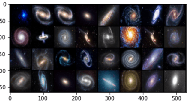
In the experiments for the remainder of this post we use a very small collection of images of Galaxies so that all of this work can be done on a laptop.  Figure 7 below shows a sample.   The images are 128 by 128 pixels with three color channels.  

Figure7.  Samples from the Galaxy image collection

Variational Autoencoders

A variational autoencoder is a neural network that uses an encoder network to reduce data samples to a lower dimensional subspace.   A decoder network takes samples from this hypothetical latent space and uses it to regenerate the samples.  The decoder becomes a means to map a uniform distribution on this latent space into the probability distribution of our samples.  In our case, the encoder has a linear map from the 49152 element input down to a vector of length 500.   This is then mapped by a  500 by 50 linear transforms down to two vectors of length 50.  The decoder does a renormalization step to produce a single vector of length 50 representing our latent space vector.   This is expanded by two linear transformations are a relu map back to length 49152. After a sigmoid transformation we have the decoded image.  Figure 8 illustrates the basic architecture.

Figure 8.   The variational autoencoder.

Without going into the mathematics of how this works (for details see our previous post or the “Deep Learning for Physics Research” book or many on-line sources), the network is designed so that the encoder network generates mean (mu) and standard deviation (logvar) of the projection of the training samples in the small latent space such that the decoder network will recreate the input.  The training works by computing the loss as a combination of two terms, the mean squared error of the difference between the regenerated image and the input image and Kullback-Leibler divergence between the uniform distribution and the distribution generated by the encoder. 

The Pytorch code is available as a the notebook in github.  The same github directory contains the zipped datafile).  Figure 9 illustrates the results of the encode/decode on 8 samples from the data set.   

Figure 9.   Samples of galaxy images from the training set and their reconstructions from the VAR.

An interesting experiment is to see how the robust the decoder is to changes in the selection of the latent variable input.   Figure 10 illustrates the response of the decoder when we follow a path in the latent space from one instance from the training set to another very similar image.

Figure 10.  image 0 and image 7 are samples from the training set. Images 1 through 6 are generated from points along the path between the latent variable for 0 and for 7.

Another interesting application was recently published.  In the paper “Detection of Anomalous Grapevine Berries Using Variational Autoencoders” Miranda et.al.  show how a VAR can be used to examine arial photos of vineyards to spot areas of possible diseased grapes.  

Generative Adversarial Networks (GANs)

Generative Adversarial networks were introduced by Goodfellow et, al (arXiv:1406.2661) as a way to build neural networks that can generate very good examples that match the properties of a collection of objects.

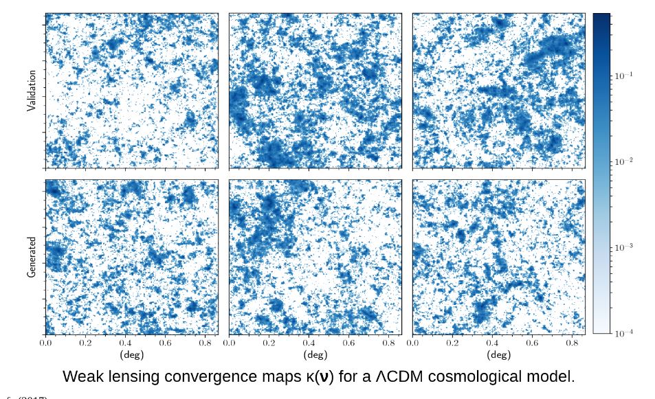
As mentioned above, artificial examples generated by autoencoder can be used as starting points for solving complex simulations.  In the case of astronomy, cosmological simulation is used to test our models of the universe. In “Creating Virtual Universes Using Generative Adversarial Networks” (arXiv:1706.02390v2 [astro-ph.IM] 17 Aug 2018) Mustafa Mustafa, et. al. demonstrates how a slightly-modified standard GAN can be used generate synthetic images of weak lensing convergence maps derived from N-body cosmological simulations.  In the remainder of this tutorial, we look at GANs.

Given a collection r of objects in Rm, a simple way to think about a generative model is as a mathematical device that transforms samples from a multivariant normal distribution Nk(0,1)  into Rm so that they look like they come from the actual distribution Pr. for our collection r.  Think of it as a function

Which maps the normal distribution into a distribution Pg  over Rm.  

In addition, assume we have a discriminator function

With the property that D(x) is the probability that x is in our collection r.   Our goal is to train G so that Pg matches Pr.   Our discriminator is trained to reject images generated by the generator while recognizing all the elements of Pr.  The generator is trained to fool the discriminator, so we have a game defined by minimax objective:

We have put a simple basic GAN from our previous post.  Running it for many epochs can occasionally get some reasonable results as shown if Figure 11.  While this looks good, it is not. Notice that it generated examples of only 3 of our samples.  This repeating of an image for different latent vectors is an example of a phenomenon called modal collapse


Figure 11.  The lack of variety in the images is called model collapse.

acGAN

There are several variations on GANs that avoid many of these problems.   One is called an acGAN for auxiliary classifier Gan developed by Augustus Odena, Christopher Olah and Jonathon Shlens.  For an acGan we assume that we have a class label for each image.   In our case the data has three categories: barred spiral  (class 0), elliptical (class 1) and spiral (class 2).   The discriminator is modified so that it not only returns the probability that the image is real, it also returns a guess at the class.  The generator takes an extra parameter to encourage it to generate an image of the class.   Let d-1 = the number of classes  then we have the functions

The discriminator is now trained to minimize the error in recognition but also the error in class recognition.  The best way to understand the details is to look at the code.   For this and the following examples we have notebooks that are slight modifications to the excellent work from the public Github site of Chen Kai Xu from Chen Kai Xu  Tsukuba University.  This notebook is here.  Figure 12 below shows the result of asking the generator to create galaxies of a given class. The G(z,0) generates good barred spirals, G(z,1) are excellent elliptical galaxies and G(z,2) are spirals.

Figure 12.  Results from asgan-new.  Generator G with random noise vector Z and class parameter for barred spiral = 0,  elliptical = 1 and spiral = 2. 

Wasserstein GAN with Gradient Penalty

The problem with modal collapse and convergence failure was, as stated above, commonly observed.  The Wasserstein GAN introduced by Martin Arjovsky , Soumith Chintala , and L´eon Bottou, directly addressed this problem.  Later  Ishaan Gulrajani, Faruk Ahmed, Martin Arjovsky, Vincent Dumoulin and Aaron Courville introduced a modification called a Gradient penalty which further improved the stability of the GAN convergence.  To accomplish this they added an additional loss term to the total loss  for training the discriminator as follows:

Setting the parameter lambda to 10.0 this was seen as an effective value for reducing to occurrence of mode collapse.  The gradient penalty value is computed using samples from straight lines connecting samples from Pr and Pg.   Figure 13 shows the result of a 32 random data vectors for the generator and the variety of responses reflect the full spectrum of the dataset.

Figure 13.   Results from Wasserstein with gradient penalty.

The notebook for wgan-gp is here.

Wasserstein Divergence for GANs

Jiqing Wu , Zhiwu Huang, Janine Thoma , Dinesh Acharya , and Luc Van Gool  introduced a variation on WGAN-gp called WGAN-div that addresses several technical constraints of WGAN-gp having to do with Lipschitz continuity not discussed here (see the paper).   They propose a better loss function for training the discriminator:

By experimental analysis the determine the best choice for the k and p hyperparameters are 2 and 6.

Figure 14 below illustrates the results after 5000 epochs of training. The notebook is here.

Figure 14.   Results from WG-div experiments.

Once again, this seems to have eliminated the modal collapse problem.  

Conclusion

This blog was written to do a better job illustrating autoencoder neural networks than our original articles.   We illustrated a denoising autoencoder, a variational autoencoder and three generative adversarial networks.  Of course, this is not the end of the innovation that has taken place in this area.  A good example of recent work is the progress made on Masked Autoencoders.  Kaiming He et. al.   published Masked Autoencoders Are Scalable Vision Learners in December 2021.  The idea is very simple and closely related to the underlying concepts used in Transformers for natural language processing like BERT or even GPT3.  Masking simply removes patches of the data and trains the network to “fill in the blanks”.   The same idea has been now applied to audio signal reconstruction. VL-BEiT from MSR is a generative vision-language foundation model that incorporates images and text. These new techniques show promise to generate more semantic richness to the results than previous methods. 

Scientific Workflow in the Cloud using Serverless Functions

Introduction

Wikipedia has a pretty good definition of workflow: an orchestrated and repeatable pattern of activity, enabled by the systematic organization of resources into processes that transform materials, provide services, or process information.   Doing Science involves the workflow of repeating and documenting experiments and the related data analysis. Consequently, managing workflow is critically important for the scientific endeavor. There have been dozens of projects that have built tools to simplify the process of specifying and managing workflow in science. We described some of these in our 2007 book “Workflows for e-Science” and another Wikipedia article gives another list of over a dozen scientific workflow system and this page lists over 200 systems. Many of these systems were so narrowly focused on a single scientific domain or set of applications that they have not seen broad adoption.   However, there are a few standouts and some of these have demonstrated they can manage serious scientific workflow.

Pegasus from ISI is the most well-known and used framework for managing science workflow.   To use it on the cloud you deploy a Condor cluster on a set of virtual machines. Once that is in place, Pegasus provides the tools you need to manage large workflow computations.   Makeflow from Notre Dame University is another example. Based on a generalization of the execution model for the old Unix Make system, Makeflow uses Condor but it also has a native distributed platform called WorkQueue. Makeflow is commonly used on large HPC Supercomputers but they also claim an implementation on AWS Lambda.

Workflow in the Cloud.

Doing scientific computing in the cloud is different from the traditional scientific data centers built around access to a large supercomputer. A primary difference is that the cloud support models of computing not associated with traditional batch computing frameworks.   The cloud is designed to support continuously running services. These may be simple web services or complex systems composed of hundreds of microservices. The cloud is designed to scale to your needs (and budget) on-demand. The largest commercial public clouds from Amazon, Google and Microsoft are based on far more than providing compute cycles. They offer services to build streaming applications, computer vision and speech AI services, scalable data analytics and database services, managing edge devices, robotics and now attached quantum processors. While there are tools to support batch computing (Microsoft Azure even has an attached Cray), the cloud is also an excellent host for interactive computational experimentation.

Christina Hoffa, et. al. “On the Use of Cloud Computing for Scientific Workflows” describe some early 2008 experiments using cloud technology for scientific workflow. The cloud of 2019 presents many possibilities they did not have access to.   Two of these are “cloud native” microservice frameworks such as Kubernetes and serverless computing models.

Kubernetes has been used for several workflow systems. An interesting example is Reana from CERN. Reana is a research data analysis platform that runs on your desktop or on a cloud Kubernetes cluster. Reana uses several workflow languages but the one that is most frequently used is CWL, the Common Workflow Language, which is rapidly becoming an industry standard.   CWL is used in a number of other cloud workflow tools including AVADOS from Veritas Genetics, a version of the popular Apache Airflow workflow tools and several other systems with implementations “in progress”.   Argo is another workflow took that is designed to work with Kubernetes.

Workflow Using Serverless Computing

Serverless computing is a natural fit for workflow management.   Serverless allows applications to run on demand without regard to compute resource reservation or management.   Serverless computations are triggered by events. Typical among the list of event types are:

  • Messages arriving on Message Queues
  • Changes in Databases
  • Changes in Document Stores
  • Service APIs being invoked
  • Device sensor data sending new updates

These event types are each central to workflow automation. AWS Lambda was the first production implementation of a serverless platform, but not the last. Implementations from Microsoft, IBM and Google are now available and the open source implementation from OpenWhisk is available for OpenStack and other platforms.

Serverless computing is built around the concept of “function as a service” where the basic unit of deployment is not a VM or container, but the code of a function.   When the function is deployed it is tied to a specific event category such as one of those listed above.    These functions are intended to be relatively light weight (not a massive memory footprint and a short execution time).   The semantics of the function execution dictate that they are stateless.   This allows many instances of the same function to be responding to events at the same time without conflict.  The function instances respond to an event, execute and terminate.   While the function itself is stateless, it can affect the state of other object during its brief execution.   It can write files, modify databases, and invoke other functions.

Workflow State Management

Most scientific workflows can be described as a directed acyclic graph where the nodes are the computational steps. An arc in the graph represents a completion of a task that signals another it may start.   For example, the first task writes a file in a storage container and that triggers an event which fires the subsequent task that is waiting for the data in the file. If the graph takes the shape of a tree where one node creates events which trigger one or more other nodes, the translation to serverless is straightforward: each node of the graph can be compiled into one function. (We show an example of this case in the next section.)

One of the challenges of using serverless computing for workflow is state management. If the “in degree” of a node is greater than one, then it requires more than one event to trigger the event.   Suppose there are two events that must happen before a node is triggered. If the function is stateless it cannot remember that the one of the conditions has already been met.  The problem is that the graph itself has state defined by which nodes have been enabled for execution. For example, Figure 1 is a CWL-like specification of such a case. NodeC cannot run until NodeA and NodeB both complete.

cwl

Figure 1. A CWL-like specification of a three step workflow where the third step requires that both the first step and second step are complete.   The first and second step can run simultaneously or in any order.

One common solution to this problem is to assume there is a persistent, stateful instance of a workflow manager that holds the graph and keeps track of its global state.   However, it is possible to manage the workflow with a single stateless function. To see how this can be done notice that in the above specification each of the step nodes requires the existence of one or more input files and the computation at that node produces one or more output files.  As shown in Figure 2 below, workflow stateless function listens to the changes to the file system (or a database).

lambda_plus_kub

Figure 2.   A workflow manager/listener function responds to events in the file system created by the execution of the applications.   As shown in the next session, if the app is small, it may be embedded in the manager, but otherwise it can be containerized and run elsewhere in the cloud.

Here we assume that the application invocations, which are shown as command-line calls in Figure 1, are either executed in the lambda function or by invocations to the application wrapped as a Docker container running as a microservice in Kubernetes. When an application terminates it deposits the output file to the file system which triggers an event for the workflow manager/listener function.

The workflow manager/listener must then decide which step nodes were affected by this event and then verify that all the conditions for that node are satisfied. For example, if the node requires two file, it much check that both are there before invoking the associated application. There is no persistent state in the manager/listener as it is all part of the file system. To run multiple workflow instances concurrently each event and file must have an instance number ID as part of its metadata.

A Simple Example of Workflow using AWS Lambda

In the following paragraphs we describe a very simple implementation of a document classification workflow using AWS Lambda. The workflow is a simple tree with two levels and our goal here is to demonstrate the levels of concurrency possible with a serverless approach. More specifically we demonstrate a system that looks for scientific documents in an AWS S3 bucket and classifies them by research topic. The results are stored in an Amazon DynamoDB table. The documents each consist of a list of “scientific phrases”. An example document is below.

“homology is part of algebraic topology”,
‘The theory of evolution animal species genes mutations’,
“the gannon-lee singularity tells us something about black holes”,
‘supercomputers are used to do very large simulations’,
‘clifford algebras and semigroup are not fields and rings’,
‘galaxies have millions of stars and some are quasars’,
‘deep learning is used to classify documents and images’,
‘surgery on compact manifolds of dimension 2 yields all possible embedded surfaces’

(In the experiments the documents are the titles of papers drawn from ArXiv.)

The first step of the workflow classifies each statement according to basic academic field: Physics, Math, Biology and Computer Science. (Obviously there more fields than this, but this covered most of the collection we used to train the classifiers.) Once a sentence is classified as to topic it is then passed to the second stage of the workflow where it is classified as to subcategory. For example if a sentence is determined to belong to Biology, the subcategories that are recognized include Neuro, Cell Behavior, Genomics, Evolution, Subcellular, Health-Tissues&Organs and Molecular Networks. Physics sub areas are Astro, General Relativity and Quantum Gravity, Condensed Matter, High Energy, Mathematical Physics, Quantum mechanics and educational physics. Math is very hard, so the categories are simple: algebra, topology, analysis and other.   The output from the DynamoDB table for this list of statements is shown in Figure 3 below.

sample-table-output

Figure 3. Output from the sample document in an AWS DynamoDB table. The “cmain predict” column is the output of the first workflow phase and the “cpredicted” column is the output of the second phase of the workflow.

The AWS Lambda details.

A Lambda function is a very simple program that responds to an event, does some processing and exits. There is a complete command line interface to Lambda, but AWS has a very nice portal interface to build Lambda functions in a variety of standard languages.   I found the web portal far superior to the command line because it gives you great debugging feedback and easy access to you function logs that are automatically generated each time your lambda function is invoked.

The example below is a very simple Python lambda function that waits for a document to arrive in a S3 storage bucket.   When a document is placed in the bucket, the “lambda_handler” function is automatically invoked. In this simple example the function does three things.   It grabs the name of the new S3 object and the bucket name. It then opens and reads the document (as text). If the document is not text, the system throws an error and the evidence is logged in the AWS CloudWatch log file for this function. In the last step, it saves the result in a DynamoDB table called “blanklambda”.

To make this work you need to assign the correct permissions policies to the lambda function. In this case we need access to S3, the DynamoDB and the basic Lambda execution role which includes permission to create the execution logs.

To tell the system which bucket to monitor you most go to the S3 bucket you want to monitor and add to the property called “Events”. Follow the instructions to a reference to your new Lambda function.

lambda-code

In our workflow example we used 5 lambda functions: a main topic classifier, and a classifier lambda function for each of the subtopics.   It is trivial to make one Lambda function create an event that will trigger another. We send each document as a string json document encoding our list of statements.

The call function is

Lam = boto3.client("lambda",region_name="us-east-1")
resp = Lam.invoke(FunctionName="bio-function", 
                  InvocationType="RequestResponse",
                  Payload=json.dumps(statementlist))

The “bio-function” Lambda code receives the payload as a text string and convert it back to a list.

The workflow is pictured in Figure 4 below.  When a document containing a list of statements lands in S3 it invokes an instance of the workflow. The main classifier lambda function invokes one instance each of the sub-classifiers and those four are all running concurrently.   As illustrated in Figure 5, when a batch of 20 documents files land in s3 as many as 100 Lambda instances are running in parallel.

workflow

Figure 4. When a document list file lands in a specified S3 bucket it triggers the main lambda function which determines the general topic of each individual statement in the document list. The entire document is sent to each of the subtopic specialist lambda function that classifies the them into subtopics and places the result in the DynamoDB table.

multiple-lambda

Figure 5. As multiple documents land in S3 new instances of the workflow are run in parallel. A batch of 20 documents arriving all at once will generate 5*20 concurrent Lambda invocations.

AWS Lambda’s Greatest Limitation

Lambda functions are intended to be small and execute quickly.   In fact, the default execution time limit is 3 seconds, but that is easily increased. What cannot be increased beyond a is the size of the package. The limit is 230Mbytes.   To import python libraries that are not included in their basic package you must add “layers”. These layers are completely analogous to the layers in the Docker Unified File System. In the case of Python a layer is a zipped file containing the libraries you need. Unfortunately, there is only one standard library layer available for python 3 and that includes numpy and scipy.   However, for our classification algorithms we need much more.   A grossly simplified (and far less accurate) version of our classifier requires only sklearn, but that is still a large package.

It takes a bit of work to build a special Lambda layer.   To create our own version of a Scikit learn library we turn to an excellent blog “How to create an AWS Lambda Python Layer” by Lucas.    We were able to do this and have a layer that also included numpy.   Unfortunately, we could not also include the model data, but we had the lambda instance dynamically load that data from S3. Because our model is simplified the load takes less than 1 second.

We tested this with 20 document files each containing 5 documents uniformly distributed over the 4 major topics. To understand the performance, we captured time stamps at the start and end of each instance of the main Lambda invocation.   Another interesting feature of AWS Lambda execution is that the amount of CPU resource assigned to each instance of a function invocation is governed by the amount of memory you allocate to it.   We tried our experiments with two different memory configurations: 380MB and 1GB.

sklearn_both-endssklearn-1G-data

Figure 6. Each horizontal line represents the execution of one Lambda workflow for one document.   Lines are ordered by start time from bottom to top. The figure on the top show the results when the lambda memory configuration was set to 380MB. The figure on the bottom shows the results with 1GB of memory allocated (and hence more cpu resource).

The results are shown in Figure 6. There are two interesting points to note.   First, the Lambda functions do not all start at the same time.   The system seems to see that there are many events that were generated by S3 and after a brief start it launches an additional set of workflow instances. We don’t know the exact scheduling mechanism used. The other thing to notice is that the increase in memory (and CPU resource made a profound difference.   While the total duration of each execution varied up to 50% between invocations the mean execution time for the large memory case was less than half that of the small memory case. In the 1GB case the system ran all 20 documents with a speed-up of 16 over the single execution case.

Having to resort to the simplified (and far less accurate) small classifier was a disappointment.   An alternative, which in many ways is more appropriate for scientific workflows, is to use the Lambda functions as a the coordination and step-trigger mechanism and have the lambda functions invoke remote services to do the real computation.   We ran instances of our full model as docker containers on the AWS LightSail platform and replaced the local invocations to the small classifier model with remote invocations to the full model as illustrated in Figure 7.

full-service

Figure 7.   Invoking the remote classifiers as web services.

Results in this configuration were heavily dependent on the scale-out of each of the classifier service. Figure 8 illustrate the behavior.

results-standard-oregon

Figure 8. Running 20 documents simultaneously pushed to S3 using remote webservice invocations for the classification step. Once again these are ordered from bottom to top by lambda start time.

As can be seen in the diagram the fastest time using a remote service for the full classifier was nearly three times faster than the small classifier running on the lambda function.   However, the requests to the service caused a bottleneck which slowed down others.   Our version of the service ran on two servers with a very primitive random scheduler for load balance.   A better design would involve many more servers dynamically allocated to meet the demand.

Conclusion

Serverless computing is a technology that can simplify the design of some scientific workflow problems. If you can define the workflow completely in terms of the occurrence of specific triggers and the graph of the execution is a simple tree, it is easy to setup a collection of function that will be triggered by the appropriate events. If the events don’t happen, the workflow is not run and you do not have to pay for servers to host it. (The example from the previous section was designed, debugged on AWS over a few weeks and run many times. The total bill was about $5.)

There are two downsides to using serverless as part of a workflow execution engine.

  1. The complexity of handling a workflow consisting of a complex non-tree DAG is large. A possible solution to this was described in Figure 2 and the accompanying text. The task of compiling a general CWL specification into such a workflow manager/listener is non-trivial because CWL specification can be very complex.
  2. A topic that was only briefly discussed here is how to get a Lambda function to execute the actual application code at each step.   In most workflow systems the work steps are command line invoked applications that take input files and produce output files. To invoke these from a serverless lambda function in the cloud requires that each worker application is rendered as a service that can be invoked from the lambda function. This can be done by containerizing the applications and deploying them in pods on Kubernetes or other microservice architecture as we illustrated in Figure 2.   In other scenarios the worker applications may be submitted to a scheduler and run on a batch system.

While we only looked at AWS Lambda here we will next consider Azure functions.   More on that later.

The source code for the lambda functions used here can be found at this GitHub repo

Note: there are various tricks to getting lambda to use larger ML libraries, but we didn’t go down that road. One good example is described in a blog by Sergei on Medium. Another look at doing ML on lambda is described by Alek Glikson in this 2018 article.

Science Applications of Generative Neural Networks

Machine learning is a common tool used in all areas of science. Applications range from simple regression models used to explain the behavior of experimental data to novel applications of deep learning. One area that has emerged in the last few years is the use of generative neural networks to produce synthetic samples of data that fit the statistical profile of real data collections. Generative models are among the most interesting deep neural networks and they abound with applications in science. The important property of all generative networks is that if you train them with a sufficiently, large and coherent collection of data samples, the network can be used to generate similar samples. But when one looks at the AI literature on generative models, one can come away with the impression that they are, at best, amazing mimics that can conjure up pictures that look like the real world, but are, in fact, pure fantasy. So why do we think that they can be of value in science? There are a several reasons one would want to use them. One reason is that the alternative method to understand nature may be based on a simulation that is extremely expensive to run. Simulations are based on the mathematical expression of a theory about the world. And theories are often loaded with parameters, some of which may have known values and others we can only guess at. Given these guesses, the simulation is the experiment: does the result look like our real-world observations? On the other hand, generative models have no explicit knowledge of the theory, but they do an excellent job of capturing the statistical distribution of the observed data. Mustafa Mustafa from LBNL states,

“We think that when it comes to practical applications of generative models, such as in the case of emulating scientific data, the criterion to evaluate generative models is to study their ability to reproduce the characteristic statistics which we can measure from the original dataset.” (from Mustafa, et. al arXiv:1706.02390v2 [astro-ph.IM] 17 Aug 2018)

Generated models can be used to create “candidates” that we can use to test and fine-tune instruments designed to capture rare events. As we shall see, they have also been used to create ‘feasible’ structures that can inform us about possibilities that were not predicted by simulations. Generative models can also be trained to generate data associated with a class label and they can be effective in eliminating noise. As we shall see this can be a powerful tool in predicting outcomes when the input data is somewhat sparse such as when medical records have missing values.

Flavors of Generative Models

There are two main types of GMs and, within each type, there are dozens of interesting variations. Generalized Adversarial Networks (GANs) consist of two networks, a discriminator and a generator (the bottom part of Figure 1 below). Given a training set of data the discriminator is trained to distinguish between the training set data and fake data produced by the generator. The generator is trained to fool the discriminator. This eventually winds up in a generator which can create data that perfectly matches the data distribution of the samples. The second family are autoencoders. Again, this involved two networks (top in figure below). One is designed to encode the sample data into a low dimensional space. The other is a decoder that takes the encoded representation and attempts to recreate it. A variational autoencoder (VAEs) is one that forces the encoded representations to fit into a distribution that looks like the unit Gaussian. In this way, samples from this compact distribution can be fed to the decoder to generate new samples.var_and_gan
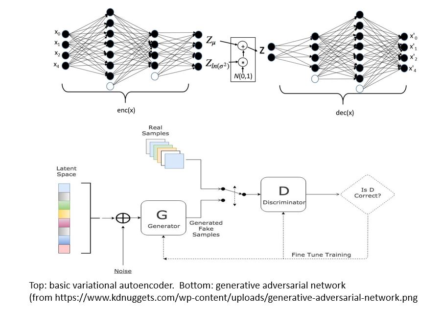
Figure 1.

Most examples of generative networks that are commonly cited involve the analysis of 2-D images based on the two opposing convolutional or similar networks.  But this need to be the case. (see “Plug & Play Generative Networks: Conditional Iterative Generation of Images in Latent Space” by Anh Nguyen, et. al. arXiv:1612.00005v2  [cs.CV]  12 Apr 2017).

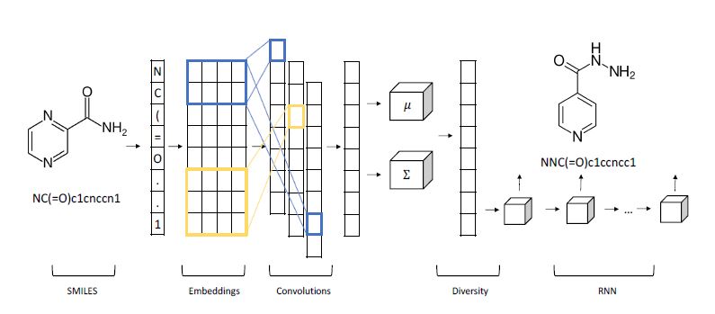
One fascinating science example we will discuss in greater detail later is by Shahar Harel and Kira Radinsky.  Shown below (Figure 2), it is a hybrid of a variational autoencoder with a convolutional encoder and recurrent neural network decoder for generating candidate chemical compounds.
VAE-with-lstm

Figure 2.  From Shahar Harel and Kira Radinsky have a different approach in “Prototype-Based Compound Discovery using Deep Generative Models” (http://kiraradinsky.com/files/acs-accelerating-prototype.pdf ).

Physics and Astronomy

Let’s start with some examples from physics and astronomy.

In statistical mechanics, Ising models provide a theoretical tool to study phase transitions in materials. The usual approach to study the behavior of this model at various temperatures is via Monte Carlo simulation. Zhaocheng Liu, Sean P. Rodrigues and Wenshan Cai from Georgia Tech in their paper “Simulating the Ising Model with a Deep Convolutional Generative Adversarial Network” (arXiv: 1710.04987v1 [cond-mat.dis-nn] 13 Oct 2017). The Ising states they generate from their network faithfully replicate the statistical properties of those generated by simulation but are also entirely new configurations not derived from previous data.

Astronomy is a topic that lends itself well to applications of generative models. Jeffrey Regier et. al. in “Celeste: Variational inference for a generative model of astronomical images” describe a detailed multi-level probabilistic model that considers both the different properties of stars and galaxies at the level of photons recorded at each pixel of the image. The purpose of the model is to infer the properties of the imaged celestial bodies. The approach is based on a variational computation similar to the VAEs described below, but far more complex in terms of the number of different modeled processes. In “Approximate Inference for Constructing Astronomical Catalogs from Images, arXiv:1803.00113v1 [stat.AP] 28 Feb 2018”, Regier and collaborators take on the problem of building catalogs of objects in thousands of images. For each imaged object there are 9 different classes of random variables that must be inferred. The goal is to compute the posterior distribution of these unobserved random variables conditional on a collection of astronomical images. They formulated a variational inference (VI) model and compared that to a Markov chain monte carlo (MCMC) method. MCMC proved to be slightly more accurate in several metrics but VI was very close. On the other hand, the variational method was 1000 times faster. It is also interesting to note that the computations were done on a Cori, the DOE supercomputer and the code was written in Julia.

Cosmological simulation is used to test our models of the universe. In “Creating Virtual Universes Using Generative Adversarial Networks” (arXiv:1706.02390v2 [astro-ph.IM] 17 Aug 2018) Mustafa Mustafa, et. al. demonstrate how a slightly-modified standard GAN can be used generate synthetic images of weak lensing convergence maps derived from N-body cosmological simulations. The results, shown in Figure 3 below, illustrate how the generated images match the validation tests. But, what is more important, the resulting images also pass a variety of statistical tests ranging from tests of the distribution of intensities to power spectrum analysis. They have made the code and data available at http://github.com/MustafaMustafa/cosmoGAN . The discussion section at the end of the paper speculates about the possibility of producing generative models that also incorporate choices for the cosmological variable that are used in the simulations.
cosmo

Figure 3.  From  Mustafa Mustafa, et. al. “Creating Virtual Universes Using Generative Adversarial Networks” (arXiv:1706.02390v2 [astro-ph.IM] 17 Aug 2018

Health Care

Medicine and health care are being transformed by the digital technology. Imaging is the most obvious place where we see advanced technology.  Our understanding of the function of proteins and RNA has exploded with high-throughput sequence analysis. Generative methods are being used here as well. Reisselman, Ingraham and Marks in “Deep generative models of genetic variation capture mutation effects” (https://www.biorxiv.org/content/biorxiv/early/2017/12/18/235655.1.full.pdf) consider the problem of how mutations to a protein disrupt it function. They developed a version of a variational autoencoder they call DeepSequence that is capable if predicting the likely effect of mutations as they evolve.

Another area of health care that is undergoing rapid change is health records. While clearly less glamourous than RNA and protein analysis, it is a part of medicine that has an impact on every patient. Our medical records are being digitized at a rapid rate and once in digital form, they can be analyzed by many machine learning tools. Hwang, Choi and Yoon in “Adversarial Training for Disease Prediction from Electronic Health Records with Missing Data” (arXiv:1711.04126v4 [cs.LG] 22 May 2018) address two important problems. First, medical records are often incomplete. They have missing value because certain test results were not correctly recorded. The process of translating old paper forms to digital artifacts can introduce additional errors. Traditional methods of dealing with this are to introduce “zero” values or “averages” to fill the gaps prior to analysis, but this is not satisfactory. Autoencoders have been shown to be very good at removing noise from data (see https://towardsdatascience.com/how-to-reduce-image-noises-by-autoencoder-65d5e6de543). Hwang and his colleagues applied this to medical records. The second thing they have done is to use a GAN to predict the disease from the “corrected” record. The type of GAN they use is an “AC-GAN” (see https://arxiv.org/pdf/1610.09585.pdf) which incorporates a class label with each training item. This allows a class label along with the random latent variable as input to force the generator to create an output similar to training elements of that class. A byproduct is a discriminator that can tell if an input has the correct class label. In their case the they are interested in if a given medical record may predict the occurrence of a tumor or not. Of course, this is far from usable as a sole diagnostic in a clinical setting, but it is a very interesting technology.

Drug Design

One exciting application of these techniques is in the design of drugs. The traditional approach is high throughput screening in which large collections of chemicals are tested against potential targets to see if any have potential therapeutic effects. Machine learning techniques have been applied to the problem for many years, but recently various deep learning method have shown surprisingly promising results. One of the inspirations for the recent work has been the recognition that molecular structures have properties similar to natural language (see Cadeddu, A, et. al.. Organic chemistry as a language and the implications of chemical linguistics for structural and retrosynthetic analyses. Angewandte Chemie 2014, 126.) More specifically, there are phrases and grammar rules in chemical compounds that have statistical properties not unlike natural language. There is a standard string representation called SMILES that an be used to illustrate these properties. SMILES representations describe atoms and their bonds and valences based on a depth-first tree traversal of a chemical graph. In modern machine learning, language structure and language tasks such as machine natural language translation are aided using recurrent neural networks. As we illustrated in our book, an RNN trained with lots of business news text is capable of generating realistic sounding business news headlines from a single starting word. However close inspection reveals that the content is nonsense. However, there is no reason we cannot apply RNNs to SMILES string to see if they can generate new molecules. Fortunately, there are sanity tests that can be applied to generated SMILES string to filter out the meaningless and incorrectly structured compounds. This was done by a team at Novartis (Ertl et al. Generation of novel chemical matter using the LSTM neural network, arXiv:1712.07449) who demonstrated that these techniques could generate billions of new drug-like molecules. Anvita Gupta, Alex T. Muller, Berend J. H. Huisman, Jens A. Fuchs, Petra Schneid and Gisbert Schneider applied very similar ideas to “Generative Recurrent Networks for De Novo Drug Design” (https://www.researchgate.net/publication/320813292/downloader). They demonstrated that if they started with fragments of a drug of interest they could use the RNN and transfer learning to generate new variations that can may be very important. Another similar result is from Artur Kadurin, et. al. in “druGAN: An Advanced Generative Adversarial Autoencoder Model for de Novo Generation of New Molecules with Desired Molecular Properties in Silico.” https://pubs.acs.org/doi/10.1021/acs.molpharmaceut.7b00346

Shahar Harel and Kira Radinsky have a different approach in “Prototype-Based Compound Discovery using Deep Generative Models” (http://kiraradinsky.com/files/acs-accelerating-prototype.pdf ). There model is motivated by a standard drug discovery process which involves start with a molecule, called a prototype, with certain known useful properties and making modifications to it based on scientific experience and intuition. Harel and Radinsky designed a very interesting Variational Autoencoder shown in figure 2 above. As with several others the start with a SMILES representation of the prototype. The first step is an embedding space is generated for SMILES “language”. The characters in the prototype sequence are imbedded and fed to a layer of convolutions that allow local structures to emerge as shorter vectors that are concatenated, and a final all-to-all layer is used to generate sequence of mean and variance vectors for the prototype. This is fed to a “diversity layer” which add randomness.

The decoder is an LSTM-based recurrent network which generates the new molecule. The results they report are impressive. In a one series of experiments they took as prototypes compounds from drugs that were discovered years ago, and they were able to generate more modern variations that are known to be more powerful and effective. No known drugs were used in the training.

Summary

These are only a small sample of the research on the uses of Generative Neural networks in science.   We must now return to the question posed in the introduction:  When are these applications of neural networks advancing science?    We should first ask the question what is the role of ‘computational science’?  It was argued in the 1990s that computing and massive computational simulation had become the third paradigm of science because it was the only way to test theories for which it was impossible to design physical experiments.   Simulations of the evolution of the universe is a great example.    These simulations allowed us to test theories because they were based on theoretical models.  If the simulated universe did not look much like our own, perhaps the theory is wrong.   By 2007 Data Science was promoted as the fourth paradigm.   By mining the vast amounts of the data we generate and collect, we can certainly validating or disproving scientific claims.    But when can a network generating synthetic images qualify as science?  It is not driven by theoretical models.   Generative models can create statistical simulations that are remarkable duplicates of the statistical properties of natural systems.   In doing so they provide a space to explore that can stimulate discovery.   There are three classes of why this can be important.

  • The value of ‘life-like’ samples. In “3D convolutional GAN for fast Simulation” F. Carminati, G.  Khattak, S.  Vallecorsa make the argument that designing and testing the next generation of sensors requires test data that is too expensive to compute with simulation.  But a well-tuned GAN is able to generate the test cases that fit the right statistical model at the rate needed for deployment.
  • Medical records-based diagnosis. The work on medical records described above by Hwang shows that using a VAE to “remove noise” is statistically superior to leaving them blank or filling in averages.   Furthermore their ability to predict disease is extremely promising as science.
  • Inspiring drug discovery. The work of Harel and Radinsky show us that a VAE can expand the scope of potential drug for further study.   This is an advance in engineering if not science.

Can it replace simulation for validating models derived from theory?  Generative neural networks are not yet able to replace simulation.   But perhaps theory can evolve so that it can be tested in new ways.

Part 2. Generative Models Tutorial

Generative Models are among the most interesting deep neural networks and they abound with applications in science. There are two main types of GMs and, within each type, several interesting variations. The important property of all generative networks is that if you train them with a sufficiently, large and coherent collection of data samples, the network can be used to generate similar samples. The key here is the definition of ‘coherent’. One can say the collection is coherent if when you are presented with a new example, it should be a simple task to decide if it belongs to the collection or not. For example, if the data collection consists entirely of pictures of cats, then a picture of a dog should be, with reasonably high probability, easily recognized as an outlier and not a cat. Of course, there are always rather extreme cats that would fool most casual observers which is why we must describe our collect of objects in term of probability distributions. Let us assume our collection c is naturally represented embedded in s2 for some m. For example, images with m pixels or other high dimensional instrument data. A simple way to think about a generative model is a mathematical device that transforms samples from a multivariant normal distribution s1 into so that they look like they come from the distribution s3 for our collection c. Think of it as a function

s4

Another useful way to say this is to build another machine we can call a discriminators5

such that for s6 is probability that X is in the collection c. To make this more “discriminating” let us also insist that s8a.  In other word, the discriminator is designed to discriminate between the real c objects and the generated ones. Of course, if the Generator is really doing a good job of imitating s3 then the discriminator with this condition would be very hard to build.  In this case we would expect s8.

Generative Adversarial networks

were introduced by Goodfellow et, al (arXiv:1406.2661) as a way to build neural networks that can generate very good examples that match the properties of a collection of objects.  It works by designed two networks:  one for the generator and one for the discriminator. Define s9 to be the distribution of latent variables that the generator will map to the collection space. The idea behind the paper is to simultaneously design the discriminator and the generator as a two-player min-max game.

The discriminator is being trained to recognize object from c (thereby reducing  s10 for  s11) and pushing s13 to zero for s14.   The resulting function

s15

Represents the min-max objective for the Discriminator.

On the other hand, the generator wants to pushs13  to 1 thereby maximizing
s16 .   To do that we minimize

s17.

There are literally dozens of implementations of GANs in Tensorflow or Karas on-line.   Below is an example from one that works with 40×40 color images.   This fragment shows the step of setting up the training optimization.

#These two placeholders are used for input into the generator and discriminator, respectively.
z_in = tf.placeholder(shape=[None,128],dtype=tf.float32) #Random vector
real_in = tf.placeholder(shape=[None,40,40,3],dtype=tf.float32) #Real images
Gz = generator(z_in) #Generates images from random z vectors
Dx = discriminator(real_in) #Produces probabilities for real images
Dg = discriminator(Gz,reuse=True) #Produces probabilities for generator images
#These functions together define the optimization objective of the GAN.
d_loss = -tf.reduce_mean(tf.log(Dx) + tf.log(1.-Dg)) #This optimizes the discriminator.
g_loss = -tf.reduce_mean(tf.log(Dg)) #This optimizes the generator.
tvars = tf.trainable_variables()
#The below code is responsible for applying gradient descent to update the GAN.
trainerD = tf.train.AdamOptimizer(learning_rate=0.0002,beta1=0.5)
trainerG = tf.train.AdamOptimizer(learning_rate=0.0002,beta1=0.5)

#Only update the weights for the discriminator network.
d_grads = trainerD.compute_gradients(d_loss,tvars[9:]) 
#Only update the weights for the generator network.
g_grads = trainerG.compute_gradients(g_loss,tvars[0:9]) 
update_D = trainerD.apply_gradients(d_grads)
update_G = trainerG.apply_gradients(g_grads)

We tested this with a very small collection of images of galaxies found on the web.  There are three types: elliptical, spiral and barred spiral.  Figure 4 below shows some high-resolution samples from the collection.

(Note:  the examples in this section use pictures of galaxies, but , in terms of the discussion in the previous part of this article, these are illustrations only.  There are no scientific results; just algorithm demonstrations. )
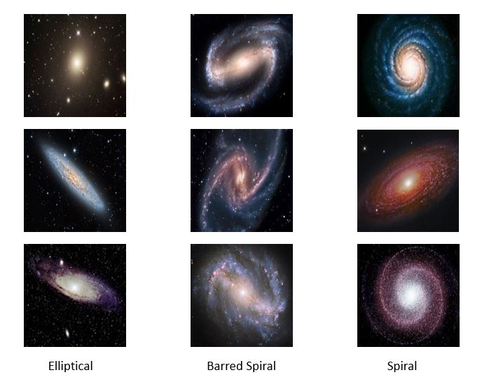
galaxy_sample

Figure 4.  Sample high-resolution galaxy images

We reduced the images to 40 by 40 and trained the GAN on this very small collection.  Drawing samples at random from the latent z-space we can now generate synthetic images.  The images we used here are only 40 by 40 pixels, so the results are not very spectacular.  As shown below, the generator is clearly able to generate elliptical and spiral forms.  In the next section we work with images that are 1024 by 1024 and get much more impressive results.
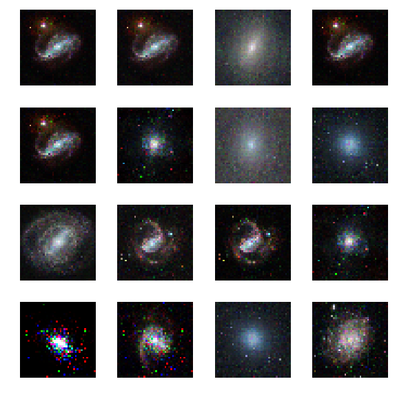
gan_40_galaxies.png

Figure 5.   Synthetic Galaxies produced by the GAN from 40×40 images.

Variational Autoencoders

The second general category generative models are based on variational autoencoders. An autoencoder transforms our collection of object representations into a space of much smaller dimension in such a way so that that representation can be used to recreate the original object with reasonably high fidelity. The system has an encoder network that creates the embedding in the smaller space and a decoder which uses that representation to regenerate an image as shown below in Figure 6.

ae

Figure 6. Generic Autoencoder

In other words, we want s18 to approximate s19 for each i in an enumeration of our collection of objects.  To train our networks we simply want to minimize the distance between s19  and s20 for each i.   If we further set up the network inputs and outputs so that they are in the range [0, 1] we can model this as a Bernouli distribution so cross entropy is a better function to minimize.  In this case the cross entropy can be calculated as

s21

(see http://www.godeep.ml/cross-entropy-likelihood-relation/  for a derivation)

A variational autoencoder differs from a general one in that we want the generator to create an embedding that is very close to a normal distribution in the embedding space.  The way we do this is to make the encoder force the encoding into a representation consisting of a mean and standard deviation.  To force it into a reasonably compact space we will force our encoder to be as close to s32  as possible. To do that we need a way to measuree how far a distribution p is from a Gaussian q. That is given by the Kullback-Leibler divergence which measures now many extra bits (or ‘nats’) are needed to convert an optimal code for distribution q into an optimal code for distribution p.

s22

If both p and q are gaussian this is easy to calculate (thought not as easy to derive).

In terms of probability distributions we can think of our encoder as s23 where x is a training image. We are going to assume  s23 is normally distributed and let s24 be  parameterized by   s25  .  Computing s26  is now easy. We call this the Latent Loss and it is

s27

(see https://stats.stackexchange.com/questions/7440/kl-divergence-between-two-univariate-gaussians for a derivation).

We now construct our encoder to produce s28 and s29 .  To sample from this latent space, we simply draw froms1 and transform it into the right space.   Our encoder and decoder networks can now be linked as follows.
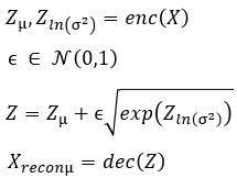
s30.JPG

the loss function is now the sum of two terms:

s31

Note: there is a Baysian approach to deriving this.  see https://jaan.io/what-is-variational-autoencoder-vae-tutorial   for an excellent discussion.

One of the interesting properties of VAEs is that they do not require massive data sets to converge.   Using our simple galaxy photo collection we trained a simple VAE.  The results showing the test inputs and the reconstructed images are illustrated below.
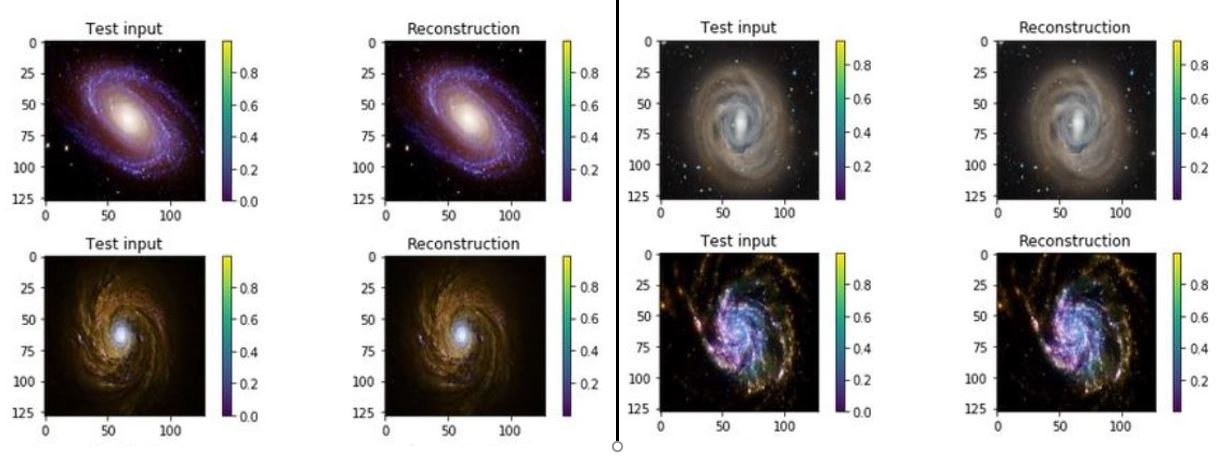
var-recon

Figure 7.   test input and reconstruction from the galaxy image collection.   These images are 1024×1024.

Using encodings of five of the images we created a path through the latent space to make the gif movie that is shown below.  While not every intermediate “galaxy” looks as good as some of the originals, it does present many reasonable “synthetic” galaxies that are on the path between two real ones.
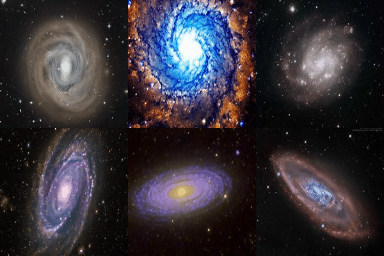
movie9

Figure 8. the “movie”.  You need to stare at it for a minute to see it evolve through synthetic and real galaxies.

The notebook for this autoencoder is available as html (see https://s3.us-east-2.amazonaws.com/a-book/autoencode-galaxy.html) and as a jupyter notebook (see https://s3.us-east-2.amazonaws.com/a-book/autoencode-galaxy.ipynb )  The compressed tarball of the galaxy images is here: https://s3.us-east-2.amazonaws.com/a-book/galaxies.tar.gz.

acGANs

The generative networks described above are just the basic variety.    One very useful addition is the Auxiliary Classifier GAN.    An acGAN allows you to incorporate knowledge about the class of the objects in your collection into the process.   For example, suppose you have labeled images such as all pictures of dogs are labeled “dog” and all pictures of cats have the label “cat”.    The original paper on this subject “Conditional Image Synthesis with Auxiliary Classifier GANs” by Oden, Olah and Shlens  shows how a GAN can be modified so that the generator can be modified so that it takes a class label in addition to the random latent variable so that it generates a new element similar to the training examples of that class. The training is augmented with an additional loss term that models the class of the training examples.

There are many more fascinating examples.   We will describe them in more detail in a later post.