Machine learning is a common tool used in all areas of science. Applications range from simple regression models used to explain the behavior of experimental data to novel applications of deep learning. One area that has emerged in the last few years is the use of generative neural networks to produce synthetic samples of data that fit the statistical profile of real data collections. Generative models are among the most interesting deep neural networks and they abound with applications in science. The important property of all generative networks is that if you train them with a sufficiently, large and coherent collection of data samples, the network can be used to generate similar samples. But when one looks at the AI literature on generative models, one can come away with the impression that they are, at best, amazing mimics that can conjure up pictures that look like the real world, but are, in fact, pure fantasy. So why do we think that they can be of value in science? There are a several reasons one would want to use them. One reason is that the alternative method to understand nature may be based on a simulation that is extremely expensive to run. Simulations are based on the mathematical expression of a theory about the world. And theories are often loaded with parameters, some of which may have known values and others we can only guess at. Given these guesses, the simulation is the experiment: does the result look like our real-world observations? On the other hand, generative models have no explicit knowledge of the theory, but they do an excellent job of capturing the statistical distribution of the observed data. Mustafa Mustafa from LBNL states,
“We think that when it comes to practical applications of generative models, such as in the case of emulating scientific data, the criterion to evaluate generative models is to study their ability to reproduce the characteristic statistics which we can measure from the original dataset.” (from Mustafa, et. al arXiv:1706.02390v2 [astro-ph.IM] 17 Aug 2018)
Generated models can be used to create “candidates” that we can use to test and fine-tune instruments designed to capture rare events. As we shall see, they have also been used to create ‘feasible’ structures that can inform us about possibilities that were not predicted by simulations. Generative models can also be trained to generate data associated with a class label and they can be effective in eliminating noise. As we shall see this can be a powerful tool in predicting outcomes when the input data is somewhat sparse such as when medical records have missing values.
Flavors of Generative Models
There are two main types of GMs and, within each type, there are dozens of interesting variations. Generalized Adversarial Networks (GANs) consist of two networks, a discriminator and a generator (the bottom part of Figure 1 below). Given a training set of data the discriminator is trained to distinguish between the training set data and fake data produced by the generator. The generator is trained to fool the discriminator. This eventually winds up in a generator which can create data that perfectly matches the data distribution of the samples. The second family are autoencoders. Again, this involved two networks (top in figure below). One is designed to encode the sample data into a low dimensional space. The other is a decoder that takes the encoded representation and attempts to recreate it. A variational autoencoder (VAEs) is one that forces the encoded representations to fit into a distribution that looks like the unit Gaussian. In this way, samples from this compact distribution can be fed to the decoder to generate new samples.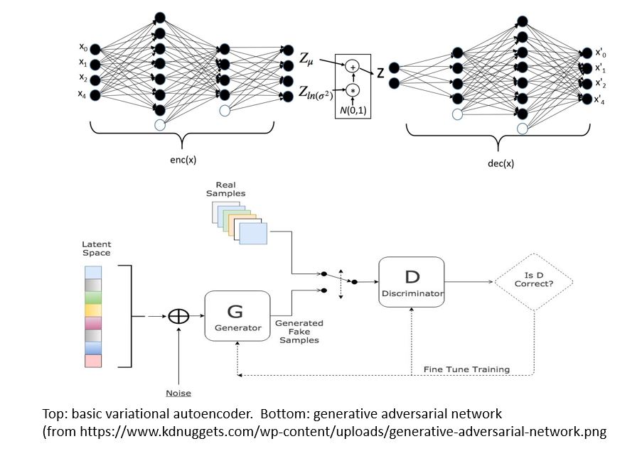
Figure 1.
Most examples of generative networks that are commonly cited involve the analysis of 2-D images based on the two opposing convolutional or similar networks. But this need to be the case. (see “Plug & Play Generative Networks: Conditional Iterative Generation of Images in Latent Space” by Anh Nguyen, et. al. arXiv:1612.00005v2 [cs.CV] 12 Apr 2017).
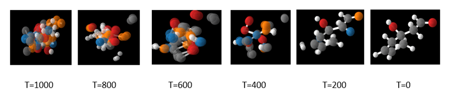
One fascinating science example we will discuss in greater detail later is by Shahar Harel and Kira Radinsky. Shown below (Figure 2), it is a hybrid of a variational autoencoder with a convolutional encoder and recurrent neural network decoder for generating candidate chemical compounds.
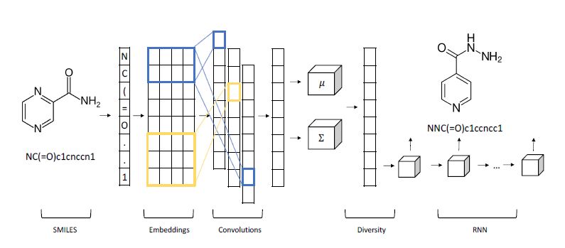
Figure 2. From Shahar Harel and Kira Radinsky have a different approach in “Prototype-Based Compound Discovery using Deep Generative Models” (http://kiraradinsky.com/files/acs-accelerating-prototype.pdf ).
Physics and Astronomy
Let’s start with some examples from physics and astronomy.
In statistical mechanics, Ising models provide a theoretical tool to study phase transitions in materials. The usual approach to study the behavior of this model at various temperatures is via Monte Carlo simulation. Zhaocheng Liu, Sean P. Rodrigues and Wenshan Cai from Georgia Tech in their paper “Simulating the Ising Model with a Deep Convolutional Generative Adversarial Network” (arXiv: 1710.04987v1 [cond-mat.dis-nn] 13 Oct 2017). The Ising states they generate from their network faithfully replicate the statistical properties of those generated by simulation but are also entirely new configurations not derived from previous data.
Astronomy is a topic that lends itself well to applications of generative models. Jeffrey Regier et. al. in “Celeste: Variational inference for a generative model of astronomical images” describe a detailed multi-level probabilistic model that considers both the different properties of stars and galaxies at the level of photons recorded at each pixel of the image. The purpose of the model is to infer the properties of the imaged celestial bodies. The approach is based on a variational computation similar to the VAEs described below, but far more complex in terms of the number of different modeled processes. In “Approximate Inference for Constructing Astronomical Catalogs from Images, arXiv:1803.00113v1 [stat.AP] 28 Feb 2018”, Regier and collaborators take on the problem of building catalogs of objects in thousands of images. For each imaged object there are 9 different classes of random variables that must be inferred. The goal is to compute the posterior distribution of these unobserved random variables conditional on a collection of astronomical images. They formulated a variational inference (VI) model and compared that to a Markov chain monte carlo (MCMC) method. MCMC proved to be slightly more accurate in several metrics but VI was very close. On the other hand, the variational method was 1000 times faster. It is also interesting to note that the computations were done on a Cori, the DOE supercomputer and the code was written in Julia.
Cosmological simulation is used to test our models of the universe. In “Creating Virtual Universes Using Generative Adversarial Networks” (arXiv:1706.02390v2 [astro-ph.IM] 17 Aug 2018) Mustafa Mustafa, et. al. demonstrate how a slightly-modified standard GAN can be used generate synthetic images of weak lensing convergence maps derived from N-body cosmological simulations. The results, shown in Figure 3 below, illustrate how the generated images match the validation tests. But, what is more important, the resulting images also pass a variety of statistical tests ranging from tests of the distribution of intensities to power spectrum analysis. They have made the code and data available at http://github.com/MustafaMustafa/cosmoGAN . The discussion section at the end of the paper speculates about the possibility of producing generative models that also incorporate choices for the cosmological variable that are used in the simulations.
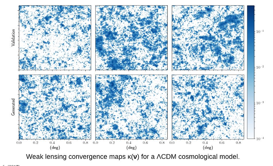
Figure 3. From Mustafa Mustafa, et. al. “Creating Virtual Universes Using Generative Adversarial Networks” (arXiv:1706.02390v2 [astro-ph.IM] 17 Aug 2018
Health Care
Medicine and health care are being transformed by the digital technology. Imaging is the most obvious place where we see advanced technology. Our understanding of the function of proteins and RNA has exploded with high-throughput sequence analysis. Generative methods are being used here as well. Reisselman, Ingraham and Marks in “Deep generative models of genetic variation capture mutation effects” (https://www.biorxiv.org/content/biorxiv/early/2017/12/18/235655.1.full.pdf) consider the problem of how mutations to a protein disrupt it function. They developed a version of a variational autoencoder they call DeepSequence that is capable if predicting the likely effect of mutations as they evolve.
Another area of health care that is undergoing rapid change is health records. While clearly less glamourous than RNA and protein analysis, it is a part of medicine that has an impact on every patient. Our medical records are being digitized at a rapid rate and once in digital form, they can be analyzed by many machine learning tools. Hwang, Choi and Yoon in “Adversarial Training for Disease Prediction from Electronic Health Records with Missing Data” (arXiv:1711.04126v4 [cs.LG] 22 May 2018) address two important problems. First, medical records are often incomplete. They have missing value because certain test results were not correctly recorded. The process of translating old paper forms to digital artifacts can introduce additional errors. Traditional methods of dealing with this are to introduce “zero” values or “averages” to fill the gaps prior to analysis, but this is not satisfactory. Autoencoders have been shown to be very good at removing noise from data (see https://towardsdatascience.com/how-to-reduce-image-noises-by-autoencoder-65d5e6de543). Hwang and his colleagues applied this to medical records. The second thing they have done is to use a GAN to predict the disease from the “corrected” record. The type of GAN they use is an “AC-GAN” (see https://arxiv.org/pdf/1610.09585.pdf) which incorporates a class label with each training item. This allows a class label along with the random latent variable as input to force the generator to create an output similar to training elements of that class. A byproduct is a discriminator that can tell if an input has the correct class label. In their case the they are interested in if a given medical record may predict the occurrence of a tumor or not. Of course, this is far from usable as a sole diagnostic in a clinical setting, but it is a very interesting technology.
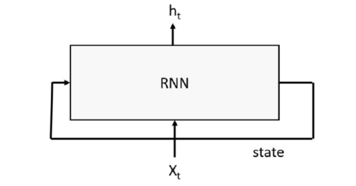
Drug Design
One exciting application of these techniques is in the design of drugs. The traditional approach is high throughput screening in which large collections of chemicals are tested against potential targets to see if any have potential therapeutic effects. Machine learning techniques have been applied to the problem for many years, but recently various deep learning method have shown surprisingly promising results. One of the inspirations for the recent work has been the recognition that molecular structures have properties similar to natural language (see Cadeddu, A, et. al.. Organic chemistry as a language and the implications of chemical linguistics for structural and retrosynthetic analyses. Angewandte Chemie 2014, 126.) More specifically, there are phrases and grammar rules in chemical compounds that have statistical properties not unlike natural language. There is a standard string representation called SMILES that an be used to illustrate these properties. SMILES representations describe atoms and their bonds and valences based on a depth-first tree traversal of a chemical graph. In modern machine learning, language structure and language tasks such as machine natural language translation are aided using recurrent neural networks. As we illustrated in our book, an RNN trained with lots of business news text is capable of generating realistic sounding business news headlines from a single starting word. However close inspection reveals that the content is nonsense. However, there is no reason we cannot apply RNNs to SMILES string to see if they can generate new molecules. Fortunately, there are sanity tests that can be applied to generated SMILES string to filter out the meaningless and incorrectly structured compounds. This was done by a team at Novartis (Ertl et al. Generation of novel chemical matter using the LSTM neural network, arXiv:1712.07449) who demonstrated that these techniques could generate billions of new drug-like molecules. Anvita Gupta, Alex T. Muller, Berend J. H. Huisman, Jens A. Fuchs, Petra Schneid and Gisbert Schneider applied very similar ideas to “Generative Recurrent Networks for De Novo Drug Design” (https://www.researchgate.net/publication/320813292/downloader). They demonstrated that if they started with fragments of a drug of interest they could use the RNN and transfer learning to generate new variations that can may be very important. Another similar result is from Artur Kadurin, et. al. in “druGAN: An Advanced Generative Adversarial Autoencoder Model for de Novo Generation of New Molecules with Desired Molecular Properties in Silico.” https://pubs.acs.org/doi/10.1021/acs.molpharmaceut.7b00346
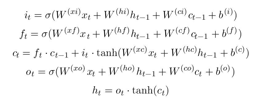
Shahar Harel and Kira Radinsky have a different approach in “Prototype-Based Compound Discovery using Deep Generative Models” (http://kiraradinsky.com/files/acs-accelerating-prototype.pdf ). There model is motivated by a standard drug discovery process which involves start with a molecule, called a prototype, with certain known useful properties and making modifications to it based on scientific experience and intuition. Harel and Radinsky designed a very interesting Variational Autoencoder shown in figure 2 above. As with several others the start with a SMILES representation of the prototype. The first step is an embedding space is generated for SMILES “language”. The characters in the prototype sequence are imbedded and fed to a layer of convolutions that allow local structures to emerge as shorter vectors that are concatenated, and a final all-to-all layer is used to generate sequence of mean and variance vectors for the prototype. This is fed to a “diversity layer” which add randomness.
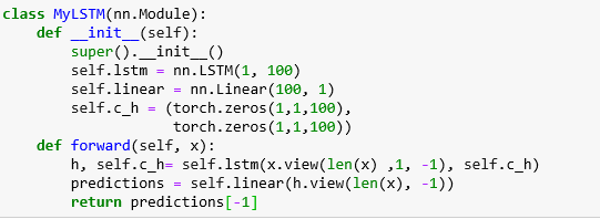
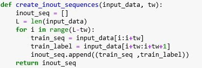
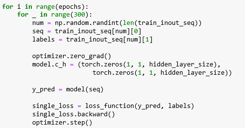
The decoder is an LSTM-based recurrent network which generates the new molecule. The results they report are impressive. In a one series of experiments they took as prototypes compounds from drugs that were discovered years ago, and they were able to generate more modern variations that are known to be more powerful and effective. No known drugs were used in the training.
Summary
These are only a small sample of the research on the uses of Generative Neural networks in science. We must now return to the question posed in the introduction: When are these applications of neural networks advancing science? We should first ask the question what is the role of ‘computational science’? It was argued in the 1990s that computing and massive computational simulation had become the third paradigm of science because it was the only way to test theories for which it was impossible to design physical experiments. Simulations of the evolution of the universe is a great example. These simulations allowed us to test theories because they were based on theoretical models. If the simulated universe did not look much like our own, perhaps the theory is wrong. By 2007 Data Science was promoted as the fourth paradigm. By mining the vast amounts of the data we generate and collect, we can certainly validating or disproving scientific claims. But when can a network generating synthetic images qualify as science? It is not driven by theoretical models. Generative models can create statistical simulations that are remarkable duplicates of the statistical properties of natural systems. In doing so they provide a space to explore that can stimulate discovery. There are three classes of why this can be important.
- The value of ‘life-like’ samples. In “3D convolutional GAN for fast Simulation” F. Carminati, G. Khattak, S. Vallecorsa make the argument that designing and testing the next generation of sensors requires test data that is too expensive to compute with simulation. But a well-tuned GAN is able to generate the test cases that fit the right statistical model at the rate needed for deployment.
- Medical records-based diagnosis. The work on medical records described above by Hwang shows that using a VAE to “remove noise” is statistically superior to leaving them blank or filling in averages. Furthermore their ability to predict disease is extremely promising as science.
- Inspiring drug discovery. The work of Harel and Radinsky show us that a VAE can expand the scope of potential drug for further study. This is an advance in engineering if not science.
Can it replace simulation for validating models derived from theory? Generative neural networks are not yet able to replace simulation. But perhaps theory can evolve so that it can be tested in new ways.
Part 2. Generative Models Tutorial
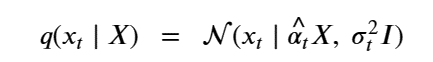
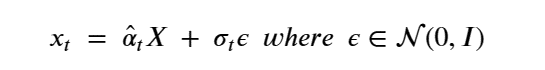
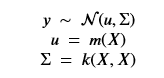
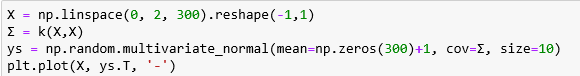
Generative Models are among the most interesting deep neural networks and they abound with applications in science. There are two main types of GMs and, within each type, several interesting variations. The important property of all generative networks is that if you train them with a sufficiently, large and coherent collection of data samples, the network can be used to generate similar samples. The key here is the definition of ‘coherent’. One can say the collection is coherent if when you are presented with a new example, it should be a simple task to decide if it belongs to the collection or not. For example, if the data collection consists entirely of pictures of cats, then a picture of a dog should be, with reasonably high probability, easily recognized as an outlier and not a cat. Of course, there are always rather extreme cats that would fool most casual observers which is why we must describe our collect of objects in term of probability distributions. Let us assume our collection c is naturally represented embedded in  for some m. For example, images with m pixels or other high dimensional instrument data. A simple way to think about a generative model is a mathematical device that transforms samples from a multivariant normal distribution
  into so that they look like they come from the distribution
  for our collection c. Think of it as a function
Another useful way to say this is to build another machine we can call a discriminator
such that for  is probability that X is in the collection c. To make this more “discriminating” let us also insist that
  . In other word, the discriminator is designed to discriminate between the real c objects and the generated ones. Of course, if the Generator is really doing a good job of imitating then the discriminator with this condition would be very hard to build. In this case we would expect
  .
.
Generative Adversarial networks
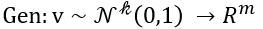
were introduced by Goodfellow et, al (arXiv:1406.2661) as a way to build neural networks that can generate very good examples that match the properties of a collection of objects. It works by designed two networks: one for the generator and one for the discriminator. Define  to be the distribution of latent variables that the generator will map to the collection space. The idea behind the paper is to simultaneously design the discriminator and the generator as a two-player min-max game.
The discriminator is being trained to recognize object from c (thereby reducing  for
for  ) and pushing
  to zero for
  . The resulting function

Represents the min-max objective for the Discriminator.
On the other hand, the generator wants to push to 1 thereby maximizing
 . To do that we minimize
 .
.
There are literally dozens of implementations of GANs in Tensorflow or Karas on-line. Below is an example from one that works with 40×40 color images. This fragment shows the step of setting up the training optimization.
#These two placeholders are used for input into the generator and discriminator, respectively.
z_in = tf.placeholder(shape=[None,128],dtype=tf.float32) #Random vector
real_in = tf.placeholder(shape=[None,40,40,3],dtype=tf.float32) #Real images
Gz = generator(z_in) #Generates images from random z vectors
Dx = discriminator(real_in) #Produces probabilities for real images
Dg = discriminator(Gz,reuse=True) #Produces probabilities for generator images
#These functions together define the optimization objective of the GAN.
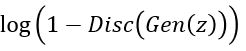
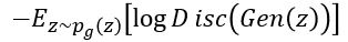
d_loss = -tf.reduce_mean(tf.log(Dx) + tf.log(1.-Dg)) #This optimizes the discriminator.
g_loss = -tf.reduce_mean(tf.log(Dg)) #This optimizes the generator.
tvars = tf.trainable_variables()
#The below code is responsible for applying gradient descent to update the GAN.
trainerD = tf.train.AdamOptimizer(learning_rate=0.0002,beta1=0.5)
trainerG = tf.train.AdamOptimizer(learning_rate=0.0002,beta1=0.5)
#Only update the weights for the discriminator network.
d_grads = trainerD.compute_gradients(d_loss,tvars[9:])
#Only update the weights for the generator network.
g_grads = trainerG.compute_gradients(g_loss,tvars[0:9])
update_D = trainerD.apply_gradients(d_grads)
update_G = trainerG.apply_gradients(g_grads)
We tested this with a very small collection of images of galaxies found on the web. There are three types: elliptical, spiral and barred spiral. Figure 4 below shows some high-resolution samples from the collection.
(Note: the examples in this section use pictures of galaxies, but , in terms of the discussion in the previous part of this article, these are illustrations only. There are no scientific results; just algorithm demonstrations. )
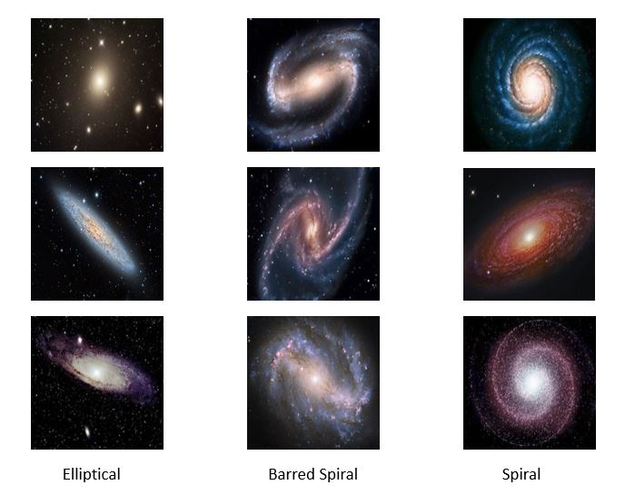
Figure 4. Sample high-resolution galaxy images
We reduced the images to 40 by 40 and trained the GAN on this very small collection. Drawing samples at random from the latent z-space we can now generate synthetic images. The images we used here are only 40 by 40 pixels, so the results are not very spectacular. As shown below, the generator is clearly able to generate elliptical and spiral forms. In the next section we work with images that are 1024 by 1024 and get much more impressive results.
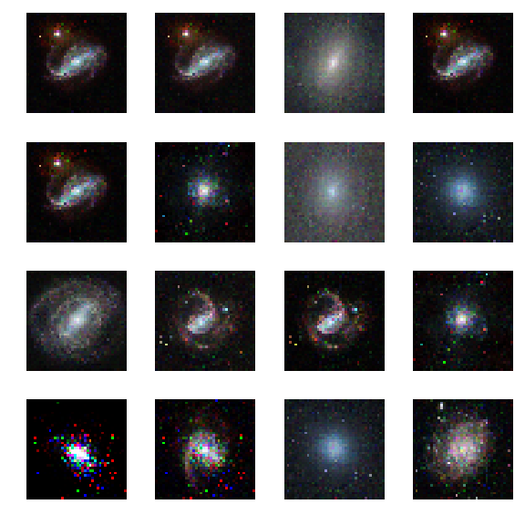
Figure 5. Synthetic Galaxies produced by the GAN from 40×40 images.
Variational Autoencoders
The second general category generative models are based on variational autoencoders. An autoencoder transforms our collection of object representations into a space of much smaller dimension in such a way so that that representation can be used to recreate the original object with reasonably high fidelity. The system has an encoder network that creates the embedding in the smaller space and a decoder which uses that representation to regenerate an image as shown below in Figure 6.

Figure 6. Generic Autoencoder
In other words, we want 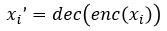 to approximate
  for each i in an enumeration of our collection of objects. To train our networks we simply want to minimize the distance between and
  for each i. If we further set up the network inputs and outputs so that they are in the range [0, 1] we can model this as a Bernouli distribution so cross entropy is a better function to minimize. In this case the cross entropy can be calculated as
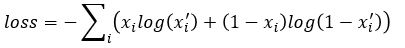
(see http://www.godeep.ml/cross-entropy-likelihood-relation/ for a derivation)
A variational autoencoder differs from a general one in that we want the generator to create an embedding that is very close to a normal distribution in the embedding space. The way we do this is to make the encoder force the encoding into a representation consisting of a mean and standard deviation. To force it into a reasonably compact space we will force our encoder to be as close to  as possible. To do that we need a way to measuree how far a distribution p is from a Gaussian q. That is given by the Kullback-Leibler divergence which measures now many extra bits (or ‘nats’) are needed to convert an optimal code for distribution q into an optimal code for distribution p.
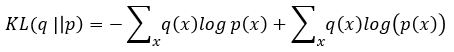
If both p and q are gaussian this is easy to calculate (thought not as easy to derive).
In terms of probability distributions we can think of our encoder as  where x is a training image. We are going to assume is normally distributed and let
  be parameterized by
  . Computing
 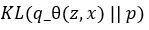 is now easy. We call this the Latent Loss and it is
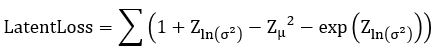
(see https://stats.stackexchange.com/questions/7440/kl-divergence-between-two-univariate-gaussians for a derivation).
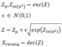
We now construct our encoder to produce  and
and  . To sample from this latent space, we simply draw from and transform it into the right space. Our encoder and decoder networks can now be linked as follows.
the loss function is now the sum of two terms:
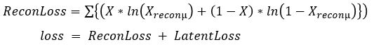
Note: there is a Baysian approach to deriving this. see https://jaan.io/what-is-variational-autoencoder-vae-tutorial for an excellent discussion.
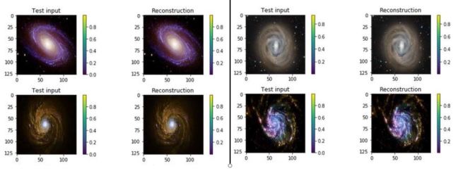
One of the interesting properties of VAEs is that they do not require massive data sets to converge. Using our simple galaxy photo collection we trained a simple VAE. The results showing the test inputs and the reconstructed images are illustrated below.
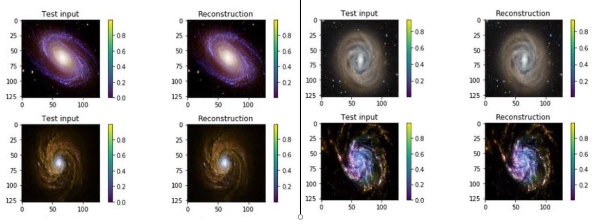
Figure 7. test input and reconstruction from the galaxy image collection. These images are 1024×1024.
Using encodings of five of the images we created a path through the latent space to make the gif movie that is shown below. While not every intermediate “galaxy” looks as good as some of the originals, it does present many reasonable “synthetic” galaxies that are on the path between two real ones.
Figure 8. the “movie”. You need to stare at it for a minute to see it evolve through synthetic and real galaxies.
The notebook for this autoencoder is available as html (see https://s3.us-east-2.amazonaws.com/a-book/autoencode-galaxy.html) and as a jupyter notebook (see https://s3.us-east-2.amazonaws.com/a-book/autoencode-galaxy.ipynb ) The compressed tarball of the galaxy images is here: https://s3.us-east-2.amazonaws.com/a-book/galaxies.tar.gz.
acGANs
The generative networks described above are just the basic variety. One very useful addition is the Auxiliary Classifier GAN. An acGAN allows you to incorporate knowledge about the class of the objects in your collection into the process. For example, suppose you have labeled images such as all pictures of dogs are labeled “dog” and all pictures of cats have the label “cat”. The original paper on this subject “Conditional Image Synthesis with Auxiliary Classifier GANs” by Oden, Olah and Shlens shows how a GAN can be modified so that the generator can be modified so that it takes a class label in addition to the random latent variable so that it generates a new element similar to the training examples of that class. The training is augmented with an additional loss term that models the class of the training examples.
There are many more fascinating examples. We will describe them in more detail in a later post.